Linear algebra is the branch of mathematics involving vectors and matrices. In particular, how vectors are transformed. Knowledge of linear algebra is essential in data science.
Linear algebra
Linear algebra allows us to understand the operations and transformations used to manipulate and extract information from data.
Examples
Deep neural networks use matrix-vector and matrix-matrix multiplication.
Natural language processing use the dot product to determine word similarity.
Least squares uses matrix inverses and matrix factorizations to compute models for predicting continuous values.
PCA (dimensionality reduction) uses the matrix factorization called the Singular Value Decomposition (SVD).
Graphs are described by adjacency matrices. Eigenvectors and eigenvalues of this matrix provide information about the graph structure.
Recommendation systems represent the interactions between users and items as a large matrix. Linear algebra is then used to compute similarities and predict missing ratings.
Linear algebra is used to implement data science algorithms efficiently and accurately.
You will not have to program linear algebra algorithms. You will use appropriate Python packages.
The goal of this lecture is to refresh the following topics:
vectors,
matrices,
operations with vectors and matrices,
eigenvectors and eigenvalues,
linear systems and least squares,
matrix factorizations.
Below is a list of very useful resources for learning about linear algebra:
Linear Algebra and Its Applications (6th edition), David C. Lay, Judi J. McDonald, and Steven R. Lay, Pearson, 2021,
Introduction to Linear Algebra (6th edition), Gilbert Strang, Wellesley-Cambridge Press, 2023,
When discussing vectors we will only consider column vectors. A row vector can always be obtained from a column vector via transposition
\[
\mathbf{x}^{T} = [x_1, x_2, \ldots, x_n].
\]
Examples of Vectors
In practice we use vectors to encode measurements or features.
a housing dataset with two features: \(\mathbf{x}=[\text{bedrooms},\text{area}]^T\) where the first component counts bedrooms and the second measures square footage.
an image patch can be represented by a long vector of pixel intensities.
Class activity (1–2 minutes): With a partner, list three different kinds of data that you can naturally represent as vectors. Share your examples with the class.
Examples: Geographic coordinates (Lat, Long, Elevation), RGB color intensities, term frequencies, sensor readings…
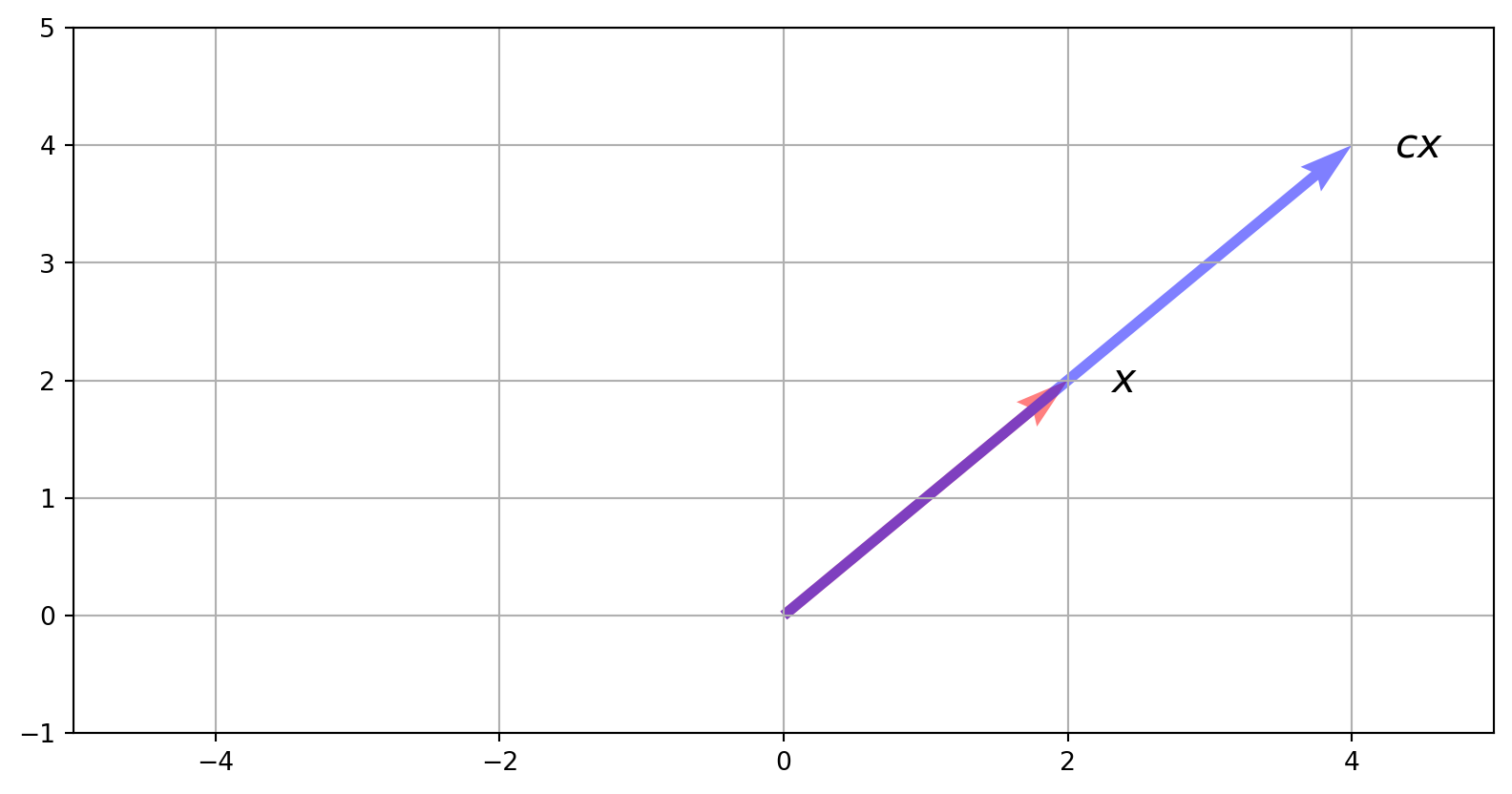
Geometric interpretation of vectors
Vectors in \(\mathbb{R}^{2}\) can be visualized as points in a 2-D plane (or arrows originating at the origin),
Vectors in \(\mathbb{R}^{3}\) can be visualized as points in a 3-D space (or arrows originating at the origin).
Although we can’t visualize vectors in \(\mathbb{R}^{n}\) for \(n>3\), we can still think of them as points in an \(n\)-dimensional space, although the curse of dimensionality comes into play (more later)
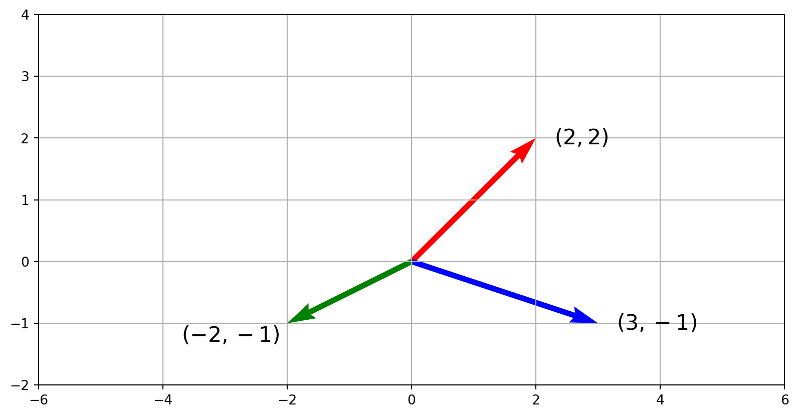
Consider these vectors in \(\mathbb{R}^{2}\) visualized in 2-D:
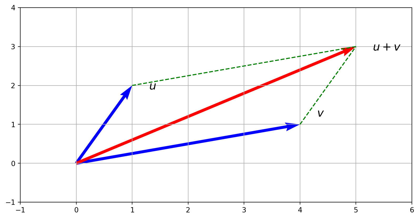
Vector addition occurs whenever you combine measurements componentwise.
For example,
if \(\mathbf{u}=[100,80]\) and \(\mathbf{v}=[20,50]\) record the number of items sold by two shops on Monday and Tuesday, then
their sum \(\mathbf{u}+\mathbf{v}=[120,130]\) gives the total items sold by both shops on those days.
Class activity (1–2 minutes): Add the vectors \(\mathbf{u}=[-1,4]\) and \(\mathbf{v}=[3,-2]\) by hand and sketch the result. Discuss how the parallelogram rule visualizes vector addition.
Element-wise multiplication
For two matrices \(A\) and \(B\) of the same dimension \(m\times n\), the Hadamard product \(A \odot B\) (sometimes \(A \circ B\)) is a matrix of the same dimension as the operands, with elements given by
\[(A \odot B)_{ij} = (A)_{ij} (B)_{ij}.\]
For matrices of different dimensions \(m\times n\) and \(p\times q\), where \(m\neq p\) or \(n\neq q\), the Hadamard product is undefined.
An example of the Hadamard product for two arbitrary \(2\times 3\) matrices:
Dot product: Let \(\mathbf{u},\mathbf{v}\in\mathbb{R}^{n}\) then the dot product is defined as \[
\mathbf{u}\cdot\mathbf{v} = \sum_{i=0}^n u_i v_i.
\]
It’s element wise multiplication, followed by summing the results.
Vector 2-norm: The 2-norm of a vector \(\mathbf{v}\in\mathbb{R}^{n}\) is defined as \[
\Vert \mathbf{v}\Vert_2 = \sqrt{\mathbf{v}\cdot\mathbf{v}} = \sqrt{\sum_{i=1}^n v_i^2}.
\]
This norm is referred to as the \(\ell_2\) norm. In these notes, the notation \(\Vert \mathbf{v} \Vert\), indicates the 2-norm.
Dot product example
Dot products and norms arise constantly in data science.
Let’s look at another numerical example.
If \(\mathbf{u}=[1,2,0]\) and \(\mathbf{v}=[3,-1,4]\), then \[
\mathbf{u}\cdot\mathbf{v} = 1\cdot 3 + 2\cdot(-1) + 0\cdot 4 = 1.
\]
norm of \(\mathbf{u}\) is \(\|\mathbf{u}\|_2 = \sqrt{1^2+2^2+0^2} = \sqrt{5}\) and the
norm of \(\mathbf{v}\) is \(\sqrt{3^2+(-1)^2+4^2}=\sqrt{26}\).
Definitions
Unit vector: A unit vector \(\mathbf{v}\) is a vector such that \(\Vert \mathbf{v} \Vert_2 = 1\).
All vectors of the form \(\frac{\mathbf{v}}{\Vert \mathbf{v} \Vert_2 }\) are unit vectors.
Distance: Let \(\mathbf{u},\mathbf{v}\in\mathbb{R}^{n}\), the distance between \(\mathbf{u}\) and \(\mathbf{v}\) is \[
\Vert \mathbf{u} - \mathbf{v} \Vert_2.
\]
Orthogonality: Two vectors \(\mathbf{u},\mathbf{v}\in\mathbb{R}^{n}\) are orthogonal if and only if \(\mathbf{u}\cdot\mathbf{v}=0\).
Angle between vectors: Let \(\mathbf{u},\mathbf{v}\in\mathbb{R}^{n}\), the angle between these vectors is \[
\cos{\theta} = \frac{\mathbf{u}\cdot\mathbf{v}}{\Vert \mathbf{u}\Vert_2 \Vert\mathbf{v}\Vert_2}.
\]
Often used as a similarity measure – “Cosine similarity”
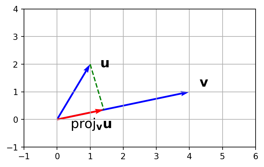
Dot product and projection
The dot product of two vectors \(\mathbf{u}, \mathbf{v}\) can be used to project \(\mathbf{u}\) onto \(\mathbf{v}\)
Observe that a right angle forms between the vectors \(\mathbf{u}\) and \(\mathbf{v}\) when \(\mathbf{u}\cdot \mathbf{v} = 0\).
And we can calculate the angle between \(\mathbf{u}\) and \(\mathbf{v}\).
Code
# Define vectors u and vu = np.array([1, 2])v = np.array([4, 1])theta = np.arccos(np.dot(u, v) / (np.linalg.norm(u) * np.linalg.norm(v)))print(f"The angle between u and v is {theta} radians or {np.degrees(theta)} degrees.")
The angle between u and v is 0.8621700546672264 radians or 49.398705354995535 degrees.
Such cosine similarities are used in natural language processing to quantify how similar two word‑embedding vectors are.
Class activity (1–2 minutes):
Compute the dot product of \(\mathbf{u}=[1,2,0]\) and \(\mathbf{v}=[3,-1,4]\).
Are the vectors orthogonal?
Next compute \(\|\mathbf{u}\|_2\), \(\|\mathbf{v}\|_2\) and the angle between them.
More Definitions
Linear dependence: A set of \(n\) vectors \(\mathbf{v}_{1}, \ldots, \mathbf{v}_{n}\in\mathbb{R}^n\) is linearly dependent if there exists scalars \(a_1,\ldots, a_n\) not all zero such that \[
\sum_{i=1}^{n} a_i \mathbf{v}_i = 0.
\]
Linear independence: The vectors \(\mathbf{v}_{1}, \ldots, \mathbf{v}_{n}\) are linearly independent if they are not linearly dependent, i.e., the equation \[
a_1 \mathbf{v}_1 + \cdots + a_n \mathbf{v}_n = 0,
\]
is only satisfied if \(a_i=0\) for \(i=1, \ldots,n\).
Span: Given a set of vectors \(V = \{\mathbf{v}_{1}, \ldots, \mathbf{v}_{n}\}\), where \(\mathbf{v}_i\in\mathbb{R}^n\), the span(V) is the set of all linear combinations of vectors in \(V\).
Let’s look at an example.
For example, the vectors \(\mathbf{v}_1=(1,1,0)\) and \(\mathbf{v}_2=(2,2,0)\) are linearly dependent because \(\mathbf{v}_2=2\mathbf{v}_1\).
In contrast, the standard basis vectors \(e_1=(1,0,0)\), \(e_2=(0,1,0)\) and \(e_3=(0,0,1)\) in \(\mathbb{R}^3\) are linearly independent, and their span is the entire three‑dimensional space.
When working with data, linear independence tells us whether a set of features carries redundant information.
Class activity (1–2 minutes): Consider the set of vectors \(\{[1,0], [0,1], [1,1]\}\) in \(\mathbb{R}^2\). Work with a neighbor to decide whether these vectors are linearly independent. What is their span? Justify your answer.
Matrices
Matrices
A matrix \(A\in\mathbb{R}^{m\times n}\) is a 2-D array of numbers
An essential concept in linear algebra is the notion of a vector space.
A vector space is a set \(V\) such that for any two vectors in the set, say \(\mathbf{u},\mathbf{v}\in V\), and any scalars \(c\) and \(d\), the linear combination \(c\mathbf{u} + d\mathbf{v}\) is also in \(V\).
In addition, a vector space must satisfy the following properties
The set of n-dimensional vectors with real numbers, i.e., \(\mathbb{R}^n\).
Given a matrix \(A\in\mathbb{R}^{m\times n}\),
the column space\(col(A)\), which is the span of all columns in the matrix \(A\) is a vector space.
The similarly defined row space is also a vector space.
Given a matrix \(A\in\mathbb{R}^{n\times n}\), the set of all solutions to the equation \(A\mathbf{x} = \mathbf{0}\) is a vector space. This space is called the null space of matrix \(A\).
The set of all \(m\times n\) matrices with real numbers is also a vector space.
The set of all polynomials of degree \(n\) is a vector space.
Important matrices
Important matrices
We introduce notation for some commonly used and important matrices.
For every \(\mathbf{A}\in\mathbb{R}^{n\times n}\), then \(\mathbf{AI} = \mathbf{IA}\).
In practice the identity matrix leaves any vector unchanged. For example, \[
\begin{bmatrix}1 & 0 \\ 0 & 1 \end{bmatrix}
\begin{bmatrix}3\\ -2 \end{bmatrix} = \begin{bmatrix}3\\ -2 \end{bmatrix}.
\] Because of this property we sometimes call \(I\) the do nothing transform.
The inverse \(A^{-1}\in\mathbb{R}^{n\times n}\) is defined as the matrix for which \[AA^{-1} = A^{-1}A = I,\]
When \(A^{-1}\) exists the matrix is said to be invertible.
Note that \((AB)^{-1} = B^{-1}A^{-1}\) for invertible \(B\in\mathbb{R}^{n\times n}\).
For example, the \(2\times 2\) matrix \[
A = \begin{bmatrix}1 & 2\\ 3 & 4\end{bmatrix}
\] has inverse \[
A^{-1} = \begin{bmatrix}-2 & 1\\ 1.5 & -0.5\end{bmatrix},
\] and one can check that \(AA^{-1} = I\) and \(A^{-1}A = I\).
Class activity (1–2 minutes): Show that \(AA^{-1} = I\) and \(A^{-1}A = I\).
A diagonal matrix \(D\in\mathbb{R}^{n\times n}\) has entries \(d_{ij}=0\) if \(i\neq j\), i.e.,
A square matrix \(Q\in\mathbb{R}^{n}\) is orthogonal if
\[QQ^{T}=Q^{T}Q=I.\]
In particular, the inverse of an orthogonal matrix is it’s transpose.
Note: Think about this in terms of matrix multiplication of rows and columns and the dot product of orthogonal vectors.
A familiar example of an orthogonal matrix is the \(2\times 2\) rotation matrix \[
R(\theta) = \begin{bmatrix} \cos \theta & -\sin \theta\\ \sin \theta & \cos \theta\end{bmatrix}.
\] For \(\theta=45^\circ\) this becomes \(\big[\tfrac{\sqrt{2}}{2}, -\tfrac{\sqrt{2}}{2}; \tfrac{\sqrt{2}}{2}, \tfrac{\sqrt{2}}{2}\big]\), and one can verify that \(R(\theta)R(\theta)^T=I\).
Orthogonal matrices preserve lengths and angles, which is why they model rigid rotations and reflections.
Class activity (1–2 minutes): Show that the \(2\times 2\) matrix \(\begin{bmatrix}0 & -1\\ 1 & 0\end{bmatrix}\) and check that it is orthogonal. What geometric transformation does it represent?
A lower triangular matrix \(L\in\mathbb{R}^{n\times n}\) is a matrix where all the entries above the main diagonal are zero
Solving a linear system \(L\mathbf{x}=\mathbf{b}\) with \(L\) lower triangular can be done efficiently by forward substitution.
For example, let \[
L = \begin{bmatrix}1 & 0\\ 2 & 3\end{bmatrix},\quad \mathbf{b} = \begin{bmatrix}1\\4\end{bmatrix}.
\] Then the system \(L\mathbf{x}=\mathbf{b}\) yields \(x_1=1\) from the first equation and \(2x_1+3x_2=4\) from the second, giving \(x_2=\tfrac{2}{3}\).
Class activity (1–2 minutes): Solve the lower triangular system \(\begin{bmatrix}1 & 0\\ -1 & 2\end{bmatrix}\mathbf{x} = \begin{bmatrix}3\\1\end{bmatrix}\) by forward substitution.
An upper triangular matrix \(U\in\mathbb{R}^{n\times n}\) is a matrix where all the entries below the main diagonal are zero
Upper triangular systems are solved by backward substitution. For example, if \[
U = \begin{bmatrix}4 & 1\\ 0 & 5\end{bmatrix},\quad \mathbf{b} = \begin{bmatrix}9\\10\end{bmatrix},
\] the equation \(U\mathbf{x}=\mathbf{b}\) implies \(5x_2=10\) so \(x_2=2\), and then \(4x_1 + x_2 =9\) gives \(x_1 = \tfrac{7}{4}\).
Class activity (1–2 minutes): Solve the upper triangular system \(\begin{bmatrix}2 & 3\\ 0 & -1\end{bmatrix}\mathbf{x} = \begin{bmatrix}7\\ -2\end{bmatrix}\) by backward substitution.
The inverse of a lower triangular matrix is itself a lower triangular matrix. This is also true for upper triangular matrices, i.e., the inverse is also upper triangular.
Eigenvalues and eigenvectors
An eigenvector of an \(n\times n\) matrix \(\mathbf{A}\) is a nonzero vector \(\mathbf{x}\) such that
\[
A\mathbf{x} = \lambda\mathbf{x}
\]
for some scalar \(\lambda.\)
The scalar \(\lambda\) is called an eigenvalue.
An \(n \times n\) matrix has at most \(n\) distinct eigenvectors and at most \(n\) distinct eigenvalues.
For example, consider the matrix \[
A = \begin{bmatrix}2 & 1\\1 & 2\end{bmatrix}.
\] It has eigenvalues \(\lambda_1=3\) and \(\lambda_2=1\) with corresponding eigenvectors \(\mathbf{v}_1=[1,1]^T\) and \(\mathbf{v}_2=[1,-1]^T\).
Eigenvectors reveal directions that the matrix stretches or compresses without changing direction.
Class activity (1–2 minutes): Verify that \(A\mathbf{v}_1 = 3\mathbf{v}_1\) and \(A\mathbf{v}_2 = 1\mathbf{v}_2\).
Matrix decompositions
We introduce here important matrix decompositions. These are useful in solving linear equations. Furthermore they play an important role in various data science applications.
LU factorization
An LU decomposition of a square matrix \(A\in\mathbb{R}^{n\times n}\) is a factorization of \(A\) into a product of matrices
\[
A = LU,
\]
where \(L\) is a lower triangular square matrix and \(U\) is an upper triangular square matrix. For example, when \(n=3\), we have
It simplifies the process of solving linear equations and is more numerically stable than computing the inverse of \(A\).
Then instad of computing the inverse of \(A\), we can solve the linear system \(A\mathbf{x}=\mathbf{b}\) in two steps:
Forward substitution: First, solve the equation \(L\mathbf{y} = \mathbf{b}\) for \(\mathbf{y}\).
Backward substitution: Then, solve \(U\mathbf{x} = \mathbf{y}\) for \(\mathbf{x}\).
This method is particularly useful because triangular matrices are much easier to work with. It can make solving linear systems faster and more efficient, especially for large matrices.
For example, consider the matrix \[
A = \begin{bmatrix}4 & 3\\6 & 3\end{bmatrix}.
\] One possible LU factorization is \[
A = LU = \begin{bmatrix}1 & 0\\ 1.5 & 1\end{bmatrix}\begin{bmatrix}4 & 3\\ 0 & -1.5\end{bmatrix}.
\] Once we have \(L\) and \(U\) we can solve \(A\mathbf{x}=\mathbf{b}\) by first solving \(L\mathbf{y}=\mathbf{b}\) and then \(U\mathbf{x}=\mathbf{y}\).
QR decomposition
A QR decomposition of a square matrix \(A\in\mathbb{R}^{n\times n}\) is a factorization of \(A\) into a product of matrices
\[
A=QR,
\] where \(Q\) is an orthogonal square matrix and \(R\) is an upper-triangular square matrix.
QR factorization is useful in solving linear systems and performing least squares fitting.
This factorization has a couple of important benefits:
Solving Linear Systems: When you’re working with a system of equations represented by \(A\mathbf{x} = \mathbf{b}\), you can substitute the QR factorization into this equation:
\[
QR\mathbf{x} = \mathbf{b}
\]
Since \(Q\) is orthogonal, you can multiply both sides by \(Q^T\) (the transpose of \(Q\)) to simplify it:
\[
R\mathbf{x} = Q^T\mathbf{b}
\]
Now, you can solve this upper triangular system for \(\mathbf{x}\) using backward substitution, which is typically easier and more stable.
Least Squares Problems: In many data science applications, you want to find the best fit line or hyperplane for your data. QR factorization is particularly useful here because it helps in minimizing the error when the system is overdetermined (more equations than unknowns). You can solve the least squares problem by leveraging the QR decomposition to find:
\[
\hat{\mathbf{x}} = R^{-1}Q^T\mathbf{b}
\]
By converting the problem into a triangular system, QR factorization often provides a more stable numerical solution than other methods, especially for poorly conditioned matrices.
As a simple example, consider the \(2\times 2\) matrix \[
A = \begin{bmatrix}1 & 1\\1 & -1\end{bmatrix}.
\] Using the Gram–Schmidt process we can factor it as \[
A = QR \quad\text{with}\quad Q = \tfrac{1}{\sqrt{2}}\begin{bmatrix}1 & 1\\1 & -1\end{bmatrix},\quad R = \sqrt{2}\begin{bmatrix}1 & 0\\ 0 & 1\end{bmatrix}.
\] Here \(Q\) has orthonormal columns and \(R\) is upper triangular.
Eigendecomposition
Let \(A\in\mathbb{R}^{n\times n}\) have \(n\) linearly independent eigenvectors \(\mathbf{x}_i\) for \(i=1,\ldots, n\), then \(A\) can be factorized as
\[
A = X\Lambda X^{-1},
\]
where the columns of matrix \(X\) are the eigenvectors of \(A\), and
In this case, the matrix \(A\) is said to be diagonalizable.
Instead of calulating \(A\mathbf{x}\) directly, we can map it by first transforming it using \(X^{-1}\) and then stretching it by \(\Lambda\) and finally transforming it using \(X\).
\[
A \mathbf{x} = X \Lambda X^{-1} \mathbf{x}
\]
We’ll use eigendecomposition in Principal Component Analysis (PCA) to reduce dimensionality in datasets while preserving as much variance as possible.
A special case occurs when \(A\) is symmetric. Recall that a matrix is symmetric when \(A = A^T.\)
In this case, it can be shown that the eigenvectors of \(A\) are all mutually orthogonal. Consequently, \(X^{-1} = X^{T}\) and we can decompose \(A\) as:
\[A = XDX^T.\]
This is known as the spectral theorem and this decomposition of \(A\) is its spectral decomposition. The eigenvalues of a matrix are also called its spectrum.
For symmetric matrices the eigenvectors can be chosen to be orthonormal, so \(X^{-1} = X^T\). In the earlier example \(A=\begin{bmatrix}2&1\\1&2\end{bmatrix}\), which is symmetric, its eigendecomposition can be written in orthonormal form as \(A = X \Lambda X^T\) with \[
X = \tfrac{1}{\sqrt{2}}\begin{bmatrix}1 & 1\\ 1 & -1\end{bmatrix},\quad \Lambda = \mathrm{diag}(3,1).
\] Because the columns of \(X\) are orthonormal, the factorization \(A = X\Lambda X^T\) is often easier to use numerically and conceptually.
Singular value decomposition
For the previous few examples, we required \(\mathbf{A}\) to be square. Now let \(A\in\mathbb{R}^{m\times n}\) with \(m>n\), then \(A\) admits a decomposition
\[
A = U\Sigma V^{T}.
\] The matrices \(U\in\mathbb{R}^{m\times m}\) and \(V\in\mathbb{R}^{n\times n}\) are orthogonal. The columns of \(U\) are the left singular vectors and the columns of \(V\) are the right singular vectors.
The matrix \(\Sigma\in\mathbb{R}^{m\times n}\) is a diagonal matrix of the form
The values \(\sigma_{ij}\) are the singular values of the matrix \(A\).
Amazingly, it can be proven that every matrix \(A\in\mathbb{R}^{m\times n}\) has a singular value decomposition.
For example, let \[
A = \begin{bmatrix}3 & 1\\ 1 & 3\end{bmatrix}.
\] This matrix has singular value decomposition \(A = U\Sigma V^T\) where the singular values are \(\sigma_1=4\) and \(\sigma_2=2\). The first singular vector (in \(U\)) points along the direction \([1,1]^T\) and corresponds to the dominant variation in the matrix. In data analysis we often keep only a few largest singular values to approximate a matrix with lower rank—a technique used in latent semantic analysis and image compression.
Class activity (1–2 minutes): Use NumPy (or by hand if you prefer) to compute the singular values of the matrix \(\begin{bmatrix}2 & 0\\ 0 & 1\end{bmatrix}\). Discuss how the singular values relate to how the matrix scales different directions.
Linear Systems and Least Squares
Linear systems of equations
A system of \(m\) linear equations in \(n\) unknowns can be written as
depending on the relationship between the rows and columns of \(A\).
Whether \(m<n\) or \(m>n\) does not by itself determine the number of solutions
the key is the rank of \(A\).
For example, the system \[
2x + y = 5,\\
x - y = 1
\] has a unique solution \((x,y)=(2,1)\).
In contrast, the system \[
2x + y = 5,\\
4x + 2y = 10
\] has infinitely many solutions because the second equation is just twice the first.
Finally the system \[
x + y = 2,\\
x + y = 3
\] has no solution because the two lines are parallel and never intersect.
When the coefficient matrix \(A\) is invertible (square and full rank), there is always a unique solution given by \(\mathbf{x}=A^{-1}\mathbf{b}\).
When \(A\) is rank deficient or when there are more equations than unknowns, a solution may not exist or there may be infinitely many solutions.
Rank deficient means that the matrix has less than \(n\) linearly independent columns.
Linear systems of equations continued
We can use matrix factorizations to help us solve a linear system of equation. We demonstrate how to do this with the LU decomposition. Observe that \[A\mathbf{x} = LU\mathbf{x} = \mathbf{b}.\]
Then
\[
\mathbf{x} = U^{-1}L^{-1}\mathbf{b}.
\]
The process of inverting \(L\) and \(U\) is called backward and forward substitution.
Least squares
In data science it is often the case that we have to solve the linear system
\[
A \mathbf{x} = \mathbf{b}.
\]
This problem may have no solution – perhaps due to noise or measurement error.
In such a case, we look for a vector \(\mathbf{x}\) such that \(A\mathbf{x}\) is a good approximation to \(\mathbf{b}.\)
The quality of the approximation can be measured using the distance from \(A\mathbf{x}\) to \(\mathbf{b},\) i.e.,
\[
\Vert A\mathbf{x} - \mathbf{b}\Vert_2.
\]
The general least-squares problem is given \(A\in\mathbb{R}^{m\times n}\) and and \(\mathbf{b}\in\mathbb{R}^{m}\), find a vector \(\hat{\mathbf{x}}\in\mathbb{R}^{n}\) such that \(\Vert A\mathbf{x}-\mathbf{b}\Vert_2\) is minimized, i.e.
This emphasizes the fact that the least squares problem is a minimization problem.
Minimizations problems are an example of a broad class of problems called optimization problems. In optimization problems we attempt to find an optimal solution that minimizes (or maximizes) a set particular set of equations (and possibly constraints).
We can connect the above minimization of the distance between vectors to the minimization of the sum of squared errors. Let \(\mathbf{y} = A\mathbf{x}\) and observe that
The above expression is the sum of squared errors. In statistics, the \(y_i\) are the estimated values and the \(b_i\) are the measured values. This is the most common measure of error used in statistics and is a key principle.
Minimizing the length of \(A\mathbf{x} - \mathbf{b}\) is equivalent to minimizing the sum of the squared errors.
We can find \(\hat{\mathbf{x}}\) using either
geometric arguments based on projections of the vector \(\mathbf{b}\),
by calculus (taking the derivative of the right-hand-side expression above and setting it equal to zero).
Either way, we obtain the result that \(\hat{\mathbf{x}}\) is the solution of:
\[A^TA\mathbf{x} = A^T\mathbf{b}.\]
This system of equations is called the normal equations.
We can prove that these equations always have at least one solution.
When \(A^TA\) is invertible, the system is said to be overdetermined. This means that there is a unique solution
\[\hat{\mathbf{x}} = (A^TA)^{-1}A^T\mathbf{b}.\]
Be aware that computing the solution using \((A^TA)^{-1}A^T\) can be numerically unstable. A more stable method is to use the QR decomposition of \(A\), i.e., \(\hat{\mathbf{x}} = R^{-1}Q^T\mathbf{b}\).
The NumPy function np.linalg.lstsq() solves the least squares problem in a stable way.
Consider the following example where the solution to the least squares problem is x=np.array([1, 1]).
# Create unit vectorunit_u = u / np.linalg.norm(u)print(f"u: {u}")print(f"Unit vector from u: {unit_u}")print(f"Norm of unit vector: {np.linalg.norm(unit_u)}")
u: [1 2 0]
Unit vector from u: [0.4472136  0.89442719 0.        ]
Norm of unit vector: 0.9999999999999999
Distance Between Vectors
Code
# Distance between vectorsdistance = np.linalg.norm(u - v)print(f"Distance between u and v: {distance}")
Distance between u and v: 5.385164807134504
Orthogonality Check
Code
# Check orthogonalitydef are_orthogonal(vec1, vec2, tolerance=1e-10):returnabs(np.dot(vec1, vec2)) < toleranceprint(f"Are u and v orthogonal? {are_orthogonal(u, v)}")# Example of orthogonal vectorsorth1 = np.array([1, 0])orth2 = np.array([0, 1])print(f"Are orth1 and orth2 orthogonal? {are_orthogonal(orth1, orth2)}")
Are u and v orthogonal? False
Are orth1 and orth2 orthogonal? True
Angle Between Vectors
Code
# Angle between vectorsdef angle_between_vectors(vec1, vec2): cos_theta = np.dot(vec1, vec2) / (np.linalg.norm(vec1) * np.linalg.norm(vec2))# Clamp to avoid numerical errors cos_theta = np.clip(cos_theta, -1.0, 1.0)return np.arccos(cos_theta)u_2d = np.array([1, 2])v_2d = np.array([4, 1])theta = angle_between_vectors(u_2d, v_2d)print(f"Angle between u and v: {theta} radians = {np.degrees(theta)} degrees")
Angle between u and v: 0.8621700546672264 radians = 49.398705354995535 degrees
Vector Projection
Code
# Project u onto vdef project_vector(u, v):return (np.dot(u, v) / np.dot(v, v)) * vprojection = project_vector(u_2d, v_2d)print(f"Projection of u onto v: {projection}")
Projection of u onto v: [1.41176471 0.35294118]
Linear Independence Check
Code
# Check linear independencedef check_linear_independence(vectors):"""Check if a set of vectors is linearly independent""" matrix = np.column_stack(vectors) rank = np.linalg.matrix_rank(matrix)return rank ==len(vectors)# Example vectorsv1 = np.array([1, 0])v2 = np.array([0, 1])v3 = np.array([1, 1])vectors = [v1, v2, v3]is_independent = check_linear_independence(vectors)print(f"Are vectors {v1}, {v2}, {v3} linearly independent? {is_independent}")
Matrix A (2x3):
[[1 2 3]
 [4 5 6]]
Matrix B (3x2):
[[ 7  8]
 [ 9 10]
 [11 12]]
A shape: (2, 3)
B shape: (3, 2)
Scalar Multiplication of Matrices
Code
# Scalar multiplicationc =2scaled_A = c * Aprint(f"Scalar multiplication:\n{scaled_A}")
Scalar multiplication:
[[ 2  4  6]
 [ 8 10 12]]
Matrix Addition
Code
# Matrix addition (matrices must have same dimensions)C = np.array([[1, 1, 1], [2, 2, 2]])matrix_sum = A + Cprint(f"Matrix addition A + C:\n{matrix_sum}")
A transpose:
[[1 4]
 [2 5]
 [3 6]]
Is matrix symmetric? True
Matrix-Vector Multiplication
Code
# Matrix-vector multiplicationx = np.array([1, 2, 3])result = A @ x # or np.dot(A, x)print(f"Matrix-vector multiplication A @ x:\n{result}")# Interpretation as linear combination of columnscol1, col2, col3 = A[:, 0], A[:, 1], A[:, 2]linear_combination = x[0]*col1 + x[1]*col2 + x[2]*col3print(f"As linear combination of columns:\n{linear_combination}")
Matrix-vector multiplication A @ x:
[14 32]
As linear combination of columns:
[14 32]
Matrix-Matrix Multiplication
Code
# Matrix-matrix multiplicationproduct = A @ Bprint(f"Matrix multiplication A @ B:\n{product}")# Element-wise calculation (for demonstration)def matrix_multiply_manual(A, B): m, n = A.shape n_b, p = B.shapeassert n == n_b, "Incompatible dimensions" C = np.zeros((m, p))for i inrange(m):for j inrange(p): C[i, j] = np.sum(A[i, :] * B[:, j])return Cmanual_product = matrix_multiply_manual(A, B)print(f"Manual matrix multiplication:\n{manual_product}")
# LU decompositionA_square = np.array([[4, 3], [6, 3]], dtype=float)P, L, U = lu(A_square)print(f"Original matrix A:\n{A_square}")print(f"P (permutation):\n{P}")print(f"L (lower triangular):\n{L}")print(f"U (upper triangular):\n{U}")print(f"Verification P@L@U:\n{P @ L @ U}")# Solve system using LU decompositiondef solve_with_lu(A, b): P, L, U = lu(A)# Solve Ly = Pb for y Pb = P @ b y = solve_triangular(L, Pb, lower=True)# Solve Ux = y for x x = solve_triangular(U, y, lower=False)return xb = np.array([7, 9])x_lu = solve_with_lu(A_square, b)print(f"Solution using LU: {x_lu}")
Original matrix A:
[[4. 3.]
 [6. 3.]]
P (permutation):
[[0. 1.]
 [1. 0.]]
L (lower triangular):
[[1.         0.        ]
 [0.66666667 1.        ]]
U (upper triangular):
[[6. 3.]
 [0. 1.]]
Verification P@L@U:
[[4. 3.]
 [6. 3.]]
Solution using LU: [1. 1.]
QR Decomposition
FIXME: This is not working.
# QR decompositionA_rect = np.array([[1, 1], [1, -1]], dtype=float)Q, R = qr(A_rect)print(f"Original matrix A:\n{A_rect}")print(f"Q (orthogonal):\n{Q}")print(f"R (upper triangular):\n{R}")print(f"Verification Q@R:\n{Q @ R}")# Verify Q is orthogonalprint(f"Q@Q.T (should be identity):\n{Q @ Q.T}")# Solve least squares using QRdef solve_least_squares_qr(A, b): Q, R = qr(A)return solve_triangular(R, Q.T @ b, lower=False)# Example overdetermined systemA_over = np.array([[1, 1], [1, 2], [1, 3]], dtype=float)b_over = np.array([2, 3, 4])x_qr = solve_least_squares_qr(A_over, b_over)print(f"Least squares solution using QR: {x_qr}")
Eigendecomposition
Code
# Eigenvalues and eigenvectorssymmetric_A = np.array([[2, 1], [1, 2]], dtype=float)eigenvalues, eigenvectors = eig(symmetric_A)print(f"Matrix A:\n{symmetric_A}")print(f"Eigenvalues: {eigenvalues}")print(f"Eigenvectors:\n{eigenvectors}")# Verify eigenvalue equation: Av = λvfor i, (lam, v) inenumerate(zip(eigenvalues, eigenvectors.T)): Av = symmetric_A @ v lambda_v = lam * vprint(f"Eigenvalue {i+1}: λ={lam:.3f}")print(f"Av = {Av}")print(f"λv = {lambda_v}")print(f"Close? {np.allclose(Av, lambda_v)}\n")# Eigendecomposition: A = XΛX^(-1)X = eigenvectorsLambda = np.diag(eigenvalues)A_reconstructed = X @ Lambda @ np.linalg.inv(X)print(f"Reconstructed A:\n{A_reconstructed}")print(f"Original A:\n{symmetric_A}")print(f"Reconstruction accurate? {np.allclose(A_reconstructed, symmetric_A)}")# For symmetric matrices: A = XΛX^Tif np.allclose(symmetric_A, symmetric_A.T): A_symmetric_recon = X @ Lambda @ X.Tprint(f"Symmetric reconstruction:\n{A_symmetric_recon}")