NN I – Gradient Descent

Introduction

Code

import numpy as np
import scipy as sp
import matplotlib.pyplot as plt
import pandas as pd
import seaborn as sns
import matplotlib as mp
import sklearn
import networkx as nx
from IPython.display import Image, HTML

import laUtilities as ut

Note

The content builds upon

Andrej Karpathy’s excellent video on building micrograd and
Understanding Deep Learning book preprint by Simone Prince
Additional sources are cited below

The “Unreasonable” Effectiveness of Deep Neural Networks

Deep Neural Networks have been effective in many applications.

Understanding Deep Learning, Simon J.D. Prince, MIT Press, 2023

Emergent Behavior in Pre-Trained Large Language Models

Emergent Abilities of Large Language Models. J. Wei et al., Oct. 26, 2022.

Theory Sometimes Follows Invention

Invention	Theory
Telescope (1608)	Optics (1650-1700)
Steam Engine (1695-1715)	Thermodynamics (1824…)
Electromagnetism (1820)	Electrodynamics (1821)
Sailboat (??)	Aerodynamics (1757), Hydrodynamics (1738)
Airplane (1885-1905)	Wing Theory (1907-1918)
Computer (1941-1945)	Computer Science (1950-1960)
Teletype (1906)	Information Theory (1948)

However, a better developed theory can lead to significant improvements in the invention.
For Neural Networks, the theory to make them work is well understood. The theory of why they work is still developing.
We’ll balance theory and application.

The Power and Limits of Deep Learning, Yann LeCun, March 2019.

Underlying Neural Networks is the minimization of a loss function.

Loss Functions for Model Fitting

Many of the machine learning models we studied this semester are based on training a parameterized model. Such a model is trained by finding the parameters which minimized the error defined through a loss function.

Here are examples we considered so far this semester:

In $k$ -means clustering, we computed $k$ cluster centroids, so that the WCSS (within cluster sum of squares) was minimized.
In linear regression, we found the parameter vector $β$ that minimized the sum of squares $‖ y - X β ‖_{2}^{2} .$
In the support vector machine, we computed a parameter vector $θ$ to minimize the classification error.

Similarly we’ll want to find good parameter settings in neural networks.

We introduce a generic approach to find good values for the parameters in problems like these.

What allows us to unify our approach to many such problems is the following:

We start by defining an error function, called a loss function, to calculate a measure of how our method is performing.
We define loss functions that are differentiable with respect to the parameters.
We use a gradient descent algorithm to find the parameters that minimize the loss function.

Thinking visually, we will see that the loss function defines a corresponding loss surface.

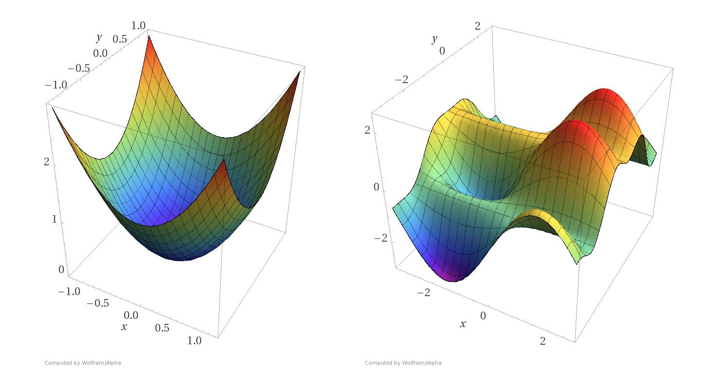
In this picture the $x -$ and $y -$ axes represent ranges of the parameters and the loss functions are plotted as surfaces.

For each parameter pair $(x, y)$ , the $z$ -axis shows the value of the loss function.

The lowest point on the surface corresponds to optimal parameters.

Notice the difference between the two kinds of surfaces.

The surface on the left corresponds to a strictly convex loss function.
A local minimum of a convex function is a global minimum.

The surface on the right corresponds to a non-convex loss function. There are local minima that are not globally minimal.

Both kinds of loss functions arise in machine learning.

For example, convex loss functions arise in

Linear regression
Logistic regression

While non-convex loss functions arise in

$k$ -means
Gaussian Mixture Modeling
Neural Networks

Gradient Descent Intuitively

The intuition of gradient descent is the following.

Imagine you are lost in the mountains and it is foggy out.

You want to find a valley, but since it is foggy, you can only see the local area around you.

What would you do?

The natural thing is:

Look around 360 degrees.
Observe in which direction the ground is sloping downward most steeply.
Take a few steps in that direction.
Repeat the process … until the ground seems to be level.

The key to this idea is formalizing the “direction of steepest descent.”

We do this by using the differentiability of the loss function. This means that the gradient, which represents the rate of spatial change, of the loss function is defined.

The (negative) of the gradient represents the direction of steepest descent.

Derivatives on Single Variable Functions

Code

import math
import numpy as np
import matplotlib.pyplot as plt
import ipywidgets as widgets
%matplotlib inline

We’ll build our understanding of the gradient by considering derivatives of single variable functions.

Let’s start with a quadratic function

$f (x) = 3 x^{2} - 4 x + 5.$

The function $f (x)$ defined in Python.

def f(x):
  return 3*x**2 - 4*x + 5

Here is a plot of $f (x)$ .

Code

import numpy as np
plt.figure(figsize=(6, 6))

xs = np.arange(-5, 5, 0.25)
ys = f(xs)
plt.plot(xs, ys)
plt.title('$f(x) = 3x^2 - 4x + 5$')
plt.show()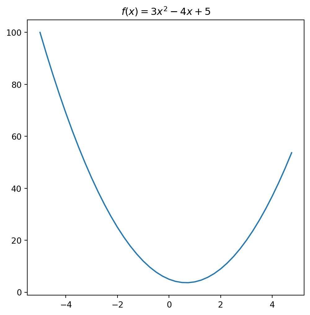

Assume that $f (x)$ is the loss function we want to minimize.

Question

What do we know about where the minimum is in terms of the slope of the curve?

Answer

The slope must necessarily be zero.

Question

How do we calculate the slope?

Answer

Calculate the derivative.

The derivative of a function $f (x)$ is denoted

$\frac{d f (x)}{d x} Leibniz’ notation,$

$f^{'} (x) Lagrange’s notation .$

You may see both notations. The nice thing about Leibniz’ notation is that it is easy to express partial derivatives. A partial derivative of a function $f (x_{1}, x_{2})$ of $2$ variables is, the derivative with respect to one of its variables. For example

$\frac{\partial f (x_{1}, x_{2})}{\partial x_{1}} = lim_{h \to 0} \frac{f (x_{1} + h, x_{2}) - f (x_{1}, x_{2})}{h} .$

A function $f (x)$ is differentiable at $x$ if

$lim_{h \to 0} \frac{f (x + h) - f (x)}{h}$

exists at $x$ . The function $f^{'} (x)$ is the value in the limit.

The derivative of our example is

$f^{'} (x) = 6 x - 4.$

You can compute this using the derivative rule $\frac{d}{d x} x^{a} = a x^{a - 1},$ for polynomial functions.

The minimum of $f (x)$ occurs at the point $x$ where $f^{'} (x) = 0$ . This is determined by solving $6 x - 4 = 0$ , which gives a value of $x = 2 / 3$ .

Plotting the point $(2 / 3, f (2 / 3))$ confirms that $x = 2 / 3$ is a minimum point.

Code

xs = np.arange(-5, 5, 0.25)
ys = f(xs)
plt.plot(xs, ys)

# Add a circle point at (2, 5)
plt.plot([2/3], [f(2/3)], 'o')

# Show the plot
plt.show()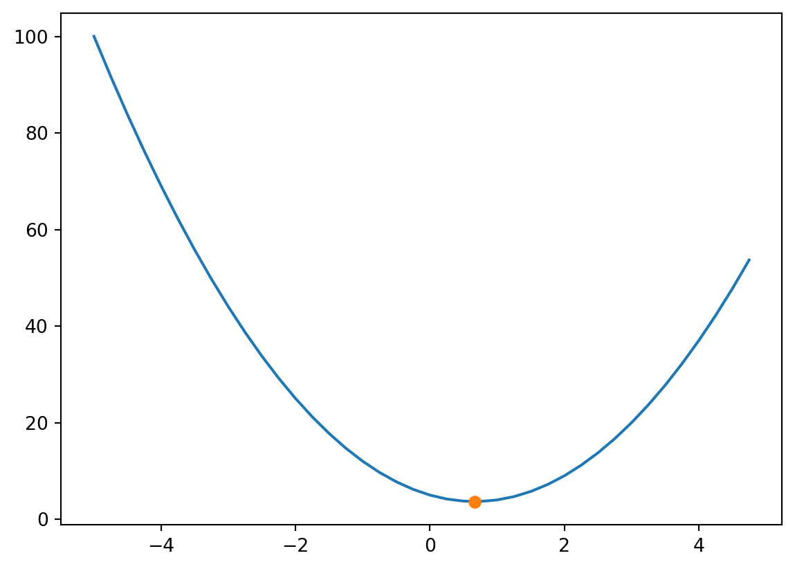

Assume $f (x)$ is differentiable. The derivative $f^{'} (x)$ is the slope of the tangent line at the point $(x, f (x))$ .

Slope of a Function

Here is an example of a tangent line at $x = - 2$ .

Code

import matplotlib.pyplot as plt
import numpy as np
import ipywidgets as widgets
from IPython.display import display

# Define the function f(x)
def f(x):
    return 3 * x ** 2 - 4 * x + 5

# Define the derivative f'(x)
def df(x):
    return 6 * x - 4

# Function to plot f(x) and its tangent line at x = x_value
def plot_with_tangent(x_value):
    # Generate x values for the function
    x = np.linspace(-5, 5, 400)
    y = f(x)

    # Compute the slope and function value at x = x_value
    slope_at_x_value = df(x_value)
    f_at_x_value = f(x_value)

    # Generate x and y values for the tangent line near x = x_value
    x_tangent = np.linspace(x_value - 2, x_value + 2, 400)
    y_tangent = f_at_x_value + slope_at_x_value * (x_tangent - x_value)

    # Create the plot
    plt.figure(figsize=(7, 4))
    plt.plot(x, y, label='$f(x) = 3x^2 - 4x + 5$')
    plt.plot(x_tangent, y_tangent, linestyle='--', label=f'Asymptotic slope of {df(x_value):.2f} at x = {x_value:.2f}')
    plt.scatter([x_value], [f_at_x_value], color='red')  # point of tangency
    plt.title('Plot of the function $f(x) = 3x^2 - 4x + 5$')
    plt.xlabel('$x$')
    plt.ylabel('$f(x)$')
    plt.grid(True)
    plt.legend()
    plt.show()

plot_with_tangent(-2)

# Create an interactive widget
# widgets.interact(plot_with_tangent, x_value=widgets.FloatSlider(value=-2, min=-5, max=5, step=0.1));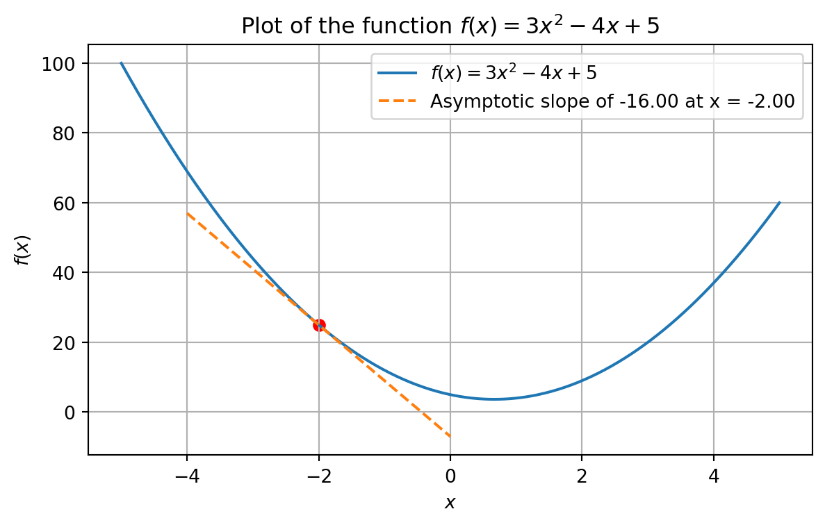

Slope Shows the Influence of $x$ on $f$

Important Note:

If the slope is negative, when $x$ increases, $f (x)$ decreases.
If the slope is positive, when $x$ decreases, $f (x)$ decreases.

Interpretation of Slope

From the graph above, consider $x = - 2$ . The value of the slope $f^{'} (2) = - 16$ . If we change the value of $x$ by a small amount $h$ , the impact on the ouptut is amplified by $- 16$ .

The slope (derivative) of a function $f (x)$ at the point $(x, f (x))$ indicates how sensitive the output is to changes in the input.

This is key to understanding how we adjust the weights of our model in order to minimize the loss function.

The Gradient

In 2 or higher dimensions, the concept of derivative generalizes to the gradient. The gradient of a multivariate function $f (x)$ , where $x = (x_{1}, \dots, x_{n}) \in R^{n}$ is the vector

$\nabla f (x) = [\begin{matrix} \frac{\partial f}{\partial x_{1}} \\ \frac{\partial f}{\partial x_{2}} \\ ⋮ \\ \frac{\partial f}{\partial x_{n}} \end{matrix}]$

It is a vector of dimension $n$ containing all the partial derivatives of the function $f (x)$ .

Gradient Descent on a Linear Regression Model

For multivariate functions, there are multiple directions to move. Similar to the 1-D case, we want to make take a step in a direction that moves us closer to the minimum value.

It turns out that if we are going to take a small step of unit length, then the gradient is the direction that maximizes the change in the loss function.

To descend, we compute the negative of the gradient. This is the idea of gradient descent for minimization.

To formalize gradient descent, consider a vector $w \in R^{n}$ . This vector $w$ contains the $n$ parameters of our model that we want to optimize.

We introduce a differentiable loss function $L (w)$ that we wish to minimize.

In linear regression, the loss function is:

$L (w) = ‖ y - \hat{y} ‖_{2}^{2},$

where $\hat{y} = X w$ is our predicted value. By substitution the loss function becomes

$L (w) = ‖ y - X w ‖_{2}^{2} .$

The gradient is the vector

$\nabla_{w} L (w) = [\begin{matrix} \frac{\partial L (w)}{\partial w_{1}} \\ \frac{\partial L (w)}{\partial w_{2}} \\ ⋮ \\ \frac{\partial L (w)}{\partial w_{n}} \end{matrix}] .$

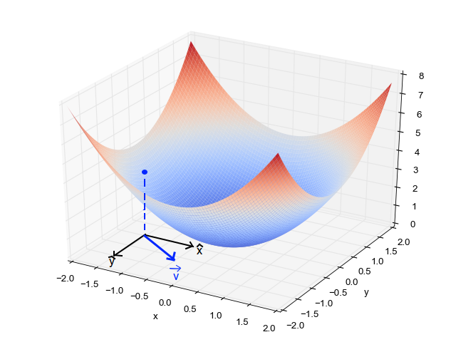
As you can see from the above figure, in general the gradient varies depending on where you are in the parameter space.

Each time we seek to improve our parameter estimates $w$ , we will take a step in the negative direction of the gradient.

… “negative direction” because the gradient specifies the direction of maximum increase – and we want to decrease the loss function.

How big a step should we take?

For step size, will use a scalar value $η$ , called the learning rate.

The learning rate is a hyperparameter that needs to be tuned for a given problem. It can also be modified adaptively as the algorithm progresses.

The gradient descent algorithm is:

Start with an initial parameter estimate $w^{0}$ .
Update: $w^{n + 1} = w^{n} - η \nabla_{w} L (w^{n})$
If not converged, go to step 2.

How do we know if the gradient descent converged?

The stopping criteria of the algorithm is:

the change in the loss is below a fixed threshold – early stopping, or
after a maximum number of iterations.

Example: Linear Regression

Assume we have the following plotted data.

Code

def centerAxes(ax):
    ax.spines['left'].set_position('zero')
    ax.spines['right'].set_color('none')
    ax.spines['bottom'].set_position('zero')
    ax.spines['top'].set_color('none')
    ax.xaxis.set_ticks_position('bottom')
    ax.yaxis.set_ticks_position('left')
    bounds = np.array([ax.axes.get_xlim(), ax.axes.get_ylim()])
    ax.plot(bounds[0][0],bounds[1][0],'')
    ax.plot(bounds[0][1],bounds[1][1],'')

n = 10
beta = np.array([1., 0.5])
ax = plt.figure(figsize = (7, 7)).add_subplot()
centerAxes(ax)
np.random.seed(1)
xlin = -10.0 + 20.0 * np.random.random(n)
y = beta[0] + (beta[1] * xlin) + np.random.randn(n)
ax.plot(xlin, y, 'ro', markersize = 10)
plt.show()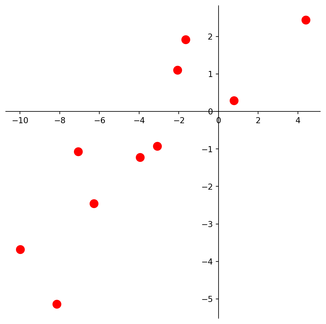

Let’s fit a least-squares line to this data.

The loss function for this problem is the least-squares error:

$L (β) = ‖ y - X β ‖_{2}^{2} .$

Rather than solve this problem using the normal equations, let’s solve it with gradient descent.

Here is the line we’d like to find.

Code

ax = plt.figure(figsize = (7, 7)).add_subplot()
centerAxes(ax)
ax.plot(xlin, y, 'ro', markersize = 10)
ax.plot(xlin, beta[0] + beta[1] * xlin, 'b-')
plt.text(-9, 3, r'$y = \beta_0 + \beta_1x$', size=20)
plt.show()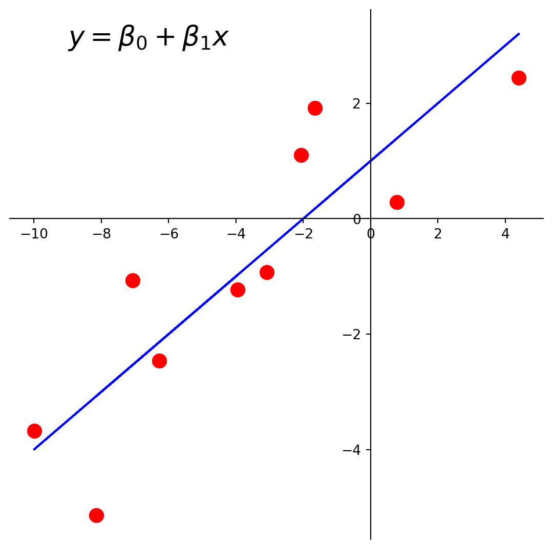

There are $n = 10$ data points, whose $x$ and $y$ values are stored in xlin and y.

First, let’s create our $X$ (design) matrix, and include a column of ones to model the intercept:

Code

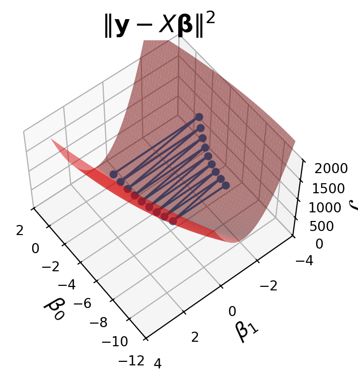
X = np.column_stack([np.ones((n, 1)), xlin])

Now, let’s visualize the loss function $L (β) = ‖ y - X β ‖_{2}^{2} .$

Code

fig = ut.three_d_figure((23, 1), '',
                        -12, 12, -4, 4, -1, 2000, 
                        figsize = (7, 7))
qf = np.array(X.T @ X)
fig.ax.view_init(azim = 60, elev = 22)
fig.plotGeneralQF(X.T @ X, -2 * (y.T @ X), y.T @ y, alpha = 0.5)
fig.ax.set_zlabel(r'$\mathcal{L}$')
fig.ax.set_xlabel(r'$\beta_0$')
fig.ax.set_ylabel(r'$\beta_1$')
fig.set_title(r'$\Vert \mathbf{y}-X\mathbf{\beta}\Vert^2$', '', 
              number_fig = False, size = 18)
# fig.save();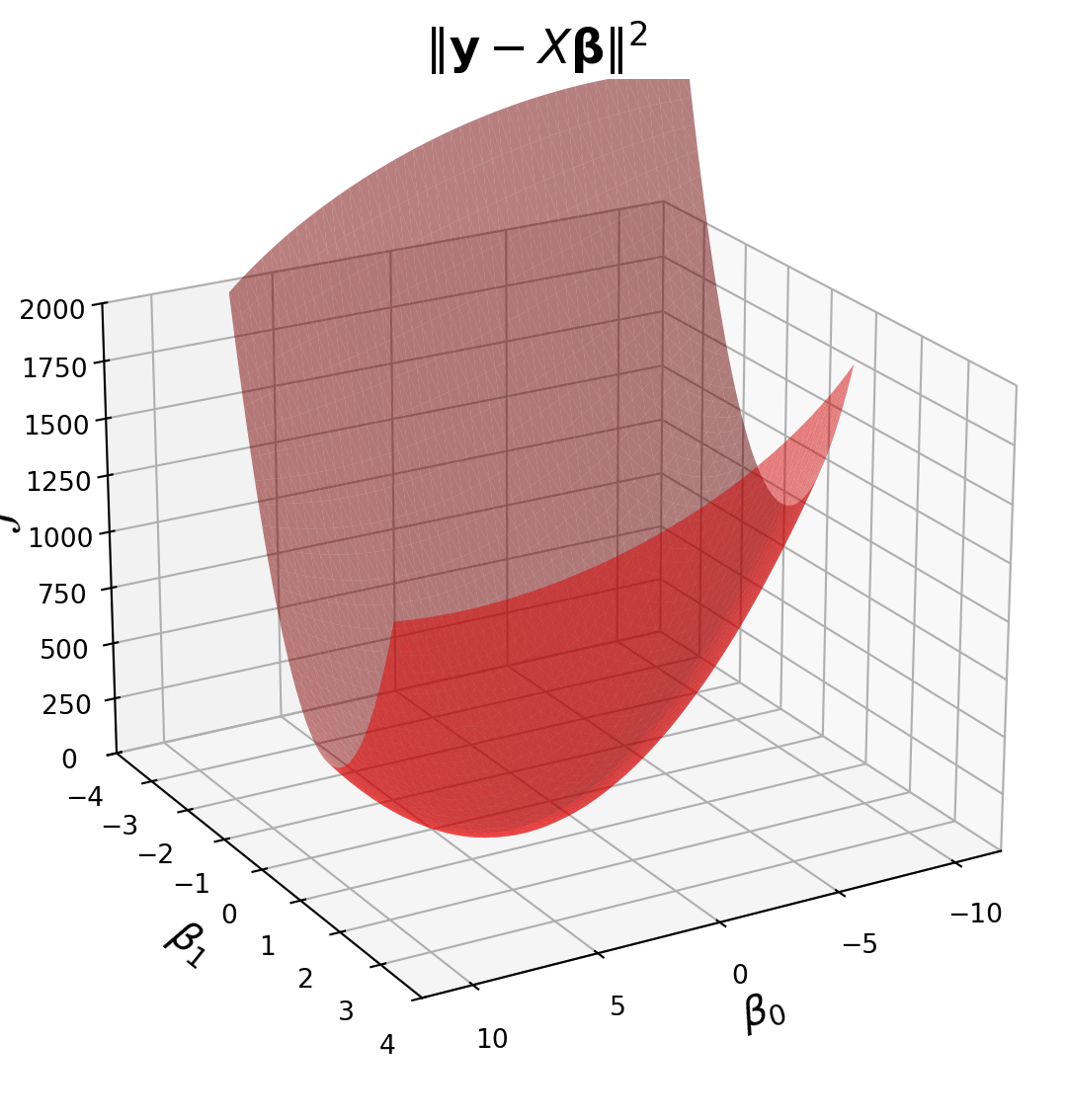

The gradient for a least squares problem is

$\nabla_{β} L (β) = X^{T} X β - X^{T} y .$

Note

For those interested in a little more insight into what these plots are showing, here is the derivation.

We start from the rule that $‖ v ‖ = \sqrt{v^{T} v}$ .

Applying this rule to our loss function:

$L (β) = ‖ y - X β ‖^{2} = β^{T} X^{T} X β - 2 β^{T} X^{T} y + y^{T} y$

The first term, $β^{T} X^{T} X β$ , is a quadratic form, and it is what makes this surface curved. As long as $X$ has independent columns, $X^{T} X$ is positive definite, so the overall shape is a paraboloid opening upward, and the surface has a unique minimum point.

To find the gradient, we can use standard calculus rules for derivates involving vectors. The rules are not complicated, but the bottom line is that in this case, you can almost use the same rules you would if $β$ were a scalar:

$\nabla_{β} L (β) = 2 X^{T} X β - 2 X^{T} y$

And by the way – since we’ve computed the derivative as a function of $β$ , instead of using gradient descent, we could simply solve for the point where the gradient is zero. This is the optimal point which we know must exist:

$\nabla_{β} L (β) = 0$

$2 X^{T} X β - 2 X^{T} y = 0$

$X^{T} X β = X^{T} y$

Which of course, are the normal equations for this linear system.

So here is our code for gradient descent:

def loss(X, y, beta):
    return np.linalg.norm(y - X @ beta) ** 2

def gradient(X, y, beta):
    return X.T @ X @ beta - X.T @ y

def gradient_descent(X, y, beta_hat, eta, nsteps = 1000):
    losses = [loss(X, y, beta_hat)]
    betas = [beta_hat]
    #
    for step in range(nsteps):
        #
        # the gradient step
        new_beta_hat = beta_hat - eta * gradient(X, y, beta_hat)
        beta_hat = new_beta_hat
        #
        # accumulate statistics
        losses.append(loss(X, y, new_beta_hat))
        betas.append(new_beta_hat)
        
    return np.array(betas), np.array(losses)

We’ll start at the point $(- 8, - 3.2)$ , i.e., $β_{0} = - 8$ , and $β_{1} = - 3.2$ .

Code

beta_start = np.array([-8, -3.2])
eta = 0.002
betas, losses = gradient_descent(X, y, beta_start, eta)

What happens to our loss function per GD iteration?

Code

plt.plot(np.log(losses), '.-')
plt.ylabel(r'$\log\mathcal{L}$', size = 14)
plt.xlabel('Iteration', size = 14)
plt.title('Improvement in Loss Per Iteration of GD', size = 16)
plt.show()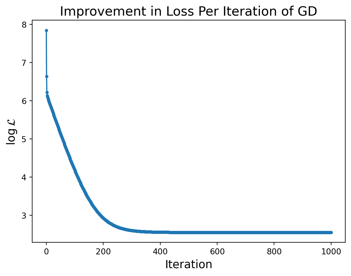

And how do the parameter values $β$ evolve?

Code

plt.plot(betas[:, 0], betas[:, 1], '.-')
plt.xlabel(r'$\beta_0$', size = 14)
plt.ylabel(r'$\beta_1$', size = 14)
plt.title(r'Evolution of $\beta$', size = 16)
plt.show()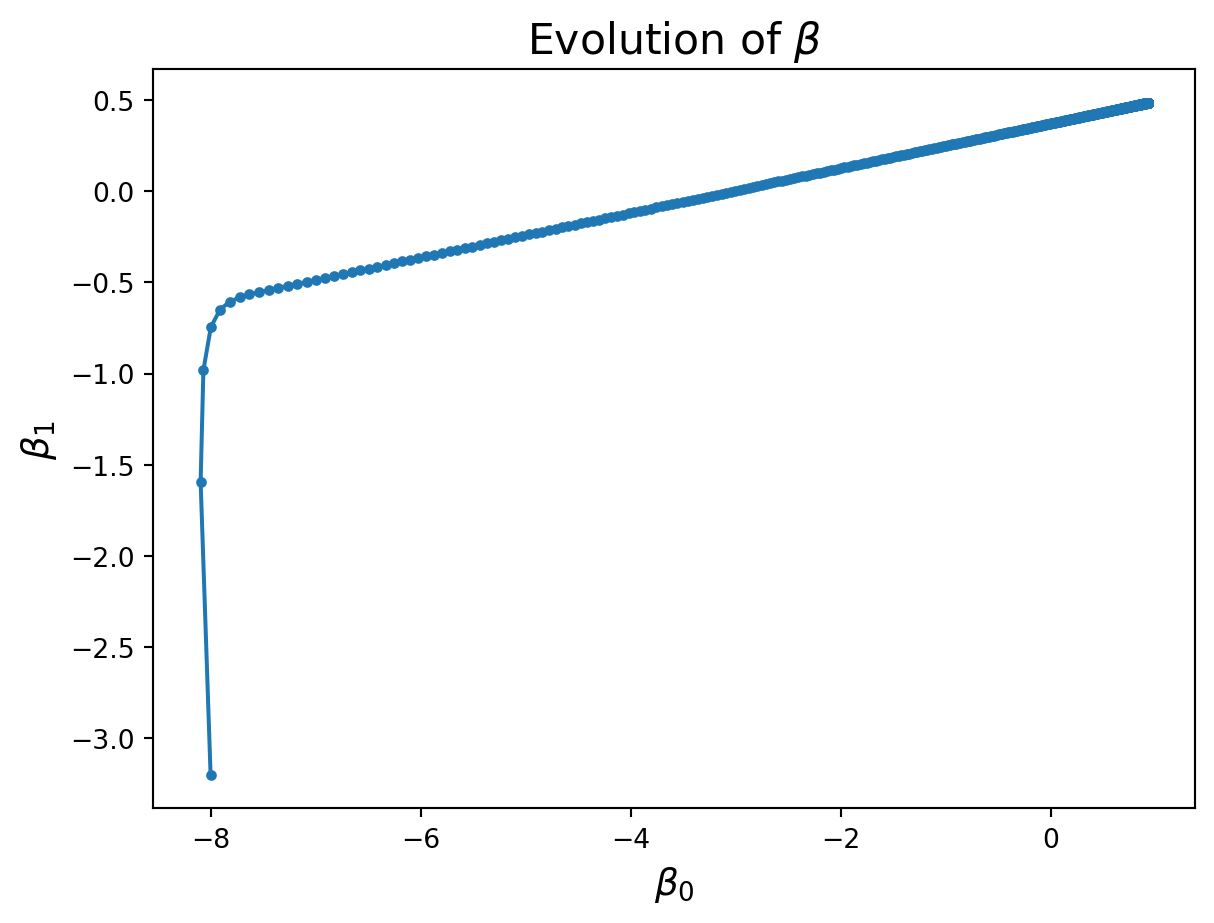

Notice that the improvement in loss decreases over time. Initially the gradient is steep and loss improves fast, while later on the gradient is shallow and loss doesn’t improve much per step.

Remember, in reality we are the person trying to find their way down the mountain in the fog.

In general, we cannot “see” the entire loss function surface.

Nonetheless, since we know what the loss surface looks like in this case, we can visualize the algorithm “moving” on that surface.

This visualization combines the last two plots into a single view.

Code

# set up view
from IPython.display import HTML
import matplotlib
import matplotlib.animation as animation
matplotlib.rcParams['animation.html'] = 'jshtml'
matplotlib.rcParams['animation.embed_limit'] = 30000000
matplotlib.rcParams['animation.html'] = 'html5'

anim_frames = np.array(list(range(10)) + [2 * x for x in range(5, 25)] + [5 * x for x in range(10, 100)])

fig = ut.three_d_figure((23, 1), 'z = 3 x1^2 + 7 x2 ^2',
                        -12, 12, -4, 4, -1, 2000, 
                        figsize = (5, 5))
plt.close()
fig.ax.view_init(azim = 60, elev = 22)
qf = np.array(X.T @ X)
fig.plotGeneralQF(X.T @ X, -2 * (y.T @ X), y.T @ y, alpha = 0.5)
fig.ax.set_zlabel(r'$\mathcal{L}$')
fig.ax.set_xlabel(r'$\beta_0$')
fig.ax.set_ylabel(r'$\beta_1$')
fig.set_title(r'$\Vert \mathbf{y}-X\mathbf{\beta}\Vert^2$', '', 
              number_fig = False, size = 18)
#
def anim(frame):
    fig.ax.plot(betas[:frame, 0], betas[:frame, 1], 'o-', zs = losses[:frame],  c = 'k', markersize = 5)
    # fig.canvas.draw()
#
# create the animation 
ani = animation.FuncAnimation(fig.fig, anim,
                       frames = anim_frames,
                       fargs = None,
                       interval = 100,
                       repeat = False)

HTML(ani.to_html5_video())

We can also see how evolution of the parameters translate to the line fitting to the data.

Code

fig, ax = plt.subplots(figsize = (5, 5))
plt.close()
centerAxes(ax)
ax.plot(xlin, y, 'ro', markersize = 10)
fit_line = ax.plot([], [])

#
#to get additional args to animate:
#def animate(angle, *fargs):
#    fargs[0].view_init(azim=angle)
def animate(frame):
    fit_line[0].set_data(xlin, betas[frame, 0] + betas[frame, 1] * xlin)
    fig.canvas.draw()
#
# create the animation 
ani = animation.FuncAnimation(fig, animate,
                       frames = anim_frames,
                       fargs=None,
                       interval=100,
                       repeat=False)


HTML(ani.to_html5_video())

Challenges in Gradient Descent

Gradient Descent can be applied to many optimization problems.

However, here are some issues to consider in practice

setting the learning rate
navigating complex loss surfaces

Learning Rate

Setting the learning rate can be a challenge. The previous learning rate was $η = 0.002$ .

Observe what happens when we set it to $η = 0.0065$ .

Code

beta_start = np.array([-8, -2])
eta = 0.0065
betas, losses = gradient_descent(X, y, beta_start, eta, nsteps = 100)

Code

plt.figure(figsize=(4, 4))
plt.plot(np.log(losses), '.-')
plt.ylabel(r'$\log\mathcal{L}$', size = 14)
plt.xlabel('Iteration', size = 14)
plt.title('Improvement in Loss Per Iteration of GD', size = 16)
plt.show()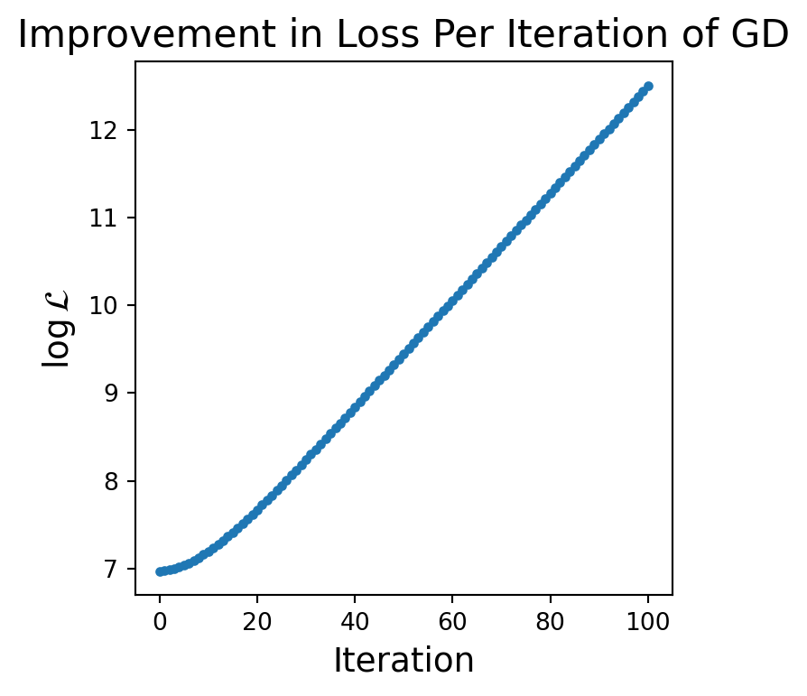

Code

plt.figure(figsize=(4, 4))
plt.plot(betas[:, 0], betas[:, 1], '.-')
plt.xlabel(r'$\beta_0$', size = 14)
plt.ylabel(r'$\beta_1$', size = 14)
plt.title(r'Evolution of $\beta$', size = 16)
plt.show()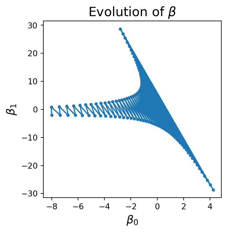

This is a total disaster. What is going on?

It is helpful to look at the progress of the algorithm using the loss surface:

Code

fig = ut.three_d_figure((23, 1), '',
                        -12, 2, -4, 4, -1, 2000, 
                        figsize = (4, 4))
qf = np.array(X.T @ X)
fig.ax.view_init(azim = 142, elev = 58)
fig.plotGeneralQF(X.T @ X, -2 * (y.T @ X), y.T @ y, alpha = 0.5)
fig.ax.set_zlabel(r'$\mathcal{L}$')
fig.ax.set_xlabel(r'$\beta_0$')
fig.ax.set_ylabel(r'$\beta_1$')
fig.set_title(r'$\Vert \mathbf{y}-X\mathbf{\beta}\Vert^2$', '', 
              number_fig = False, size = 18)
nplot = 18
fig.ax.plot(betas[:nplot, 0], betas[:nplot, 1], 'o-', zs = losses[:nplot], markersize = 5);
#

We can now see what is happening clearly.

The steps we take are too large and each step overshoots the local minimum.

The next step then lands on a portion of the surface that is steeper and in the opposite direction.

As a result the process diverges.

For an interesting comparison, try setting $η = 0.0055$ and observe the evolution of $β$ .

It is important to decrease the step size when divergence appears.

Unfortunately, on a complicated loss surface, a given step size may diverge in one location or starting point, but not in another.

Complex Loss Surfaces

The loss surface for linear regression is the best possible kind. It is strictly convex, so it has a single global minimum.

For neural networks, the loss surface is more complex.

In general, the larger the neural network, the more complex the loss surface.

And deep neural networks, especially transformers have billions of parameters.

Here’s a visualization of the loss surface for the 56 layer neural network VGG-56, from Visualizing the Loss Landscape of Neural Networks.

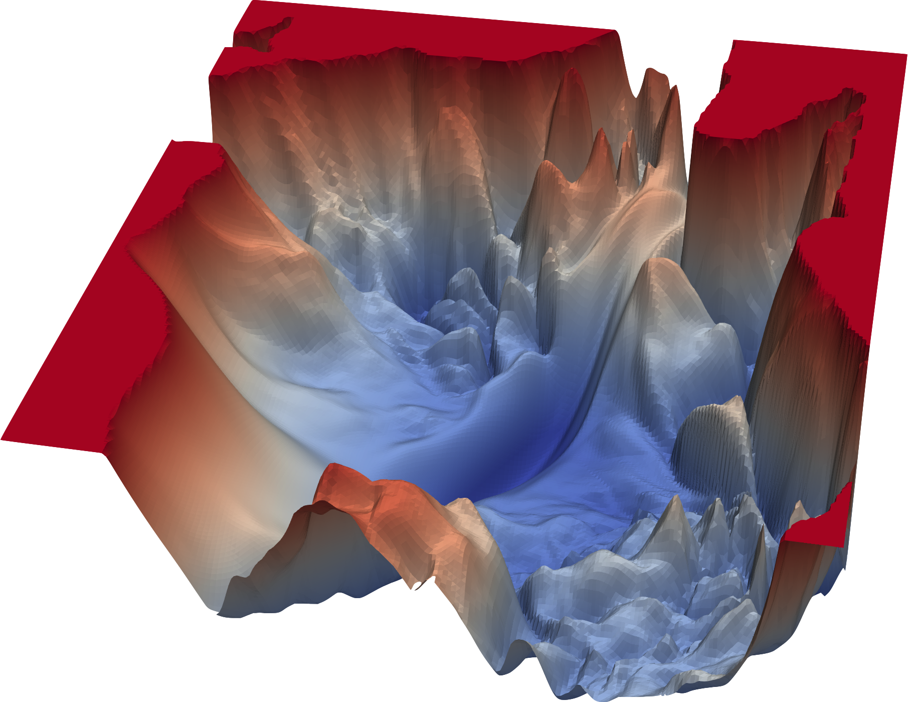
For a fun exploration, see https://losslandscape.com/explorer.

Recap

So far we applied gradient descent on a simple linear regression model.

As we’ll soon see, deep neural networks are much more complicated multi-stage models, with millions or billions of parameters to differentiate.

Fortunately, the Chain Rule from calculus gives us a relatively simple and scalable algorithm, called Back Propagation, that solves this problem.

Neuron and Neural Networks

Let’s switch gears and discuss how to construct neural networks. An _artificial neuron_is loosely modeled on a biological neuron.

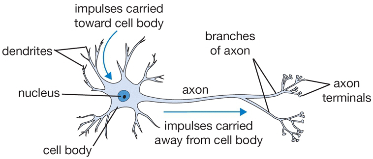
From cs231n

The dendrites carry impulses from other neurons of different distances.
Once the collective firing rate of the impulses exceed a certain threshold, the neuron fires its own pulse through the axon to other neurons.

Artificial Neuron

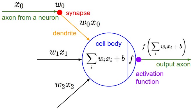
From cs231n

The more common artifical neuron

collects one or more inputs,
each multiplied by a unique weight,
sums the weighted inputs,
adds a bias,
then applies a nonlinear activation function.

Multi-Layer Perceptron (MLP) or Fully Connected Network (FCN)

From cs231n

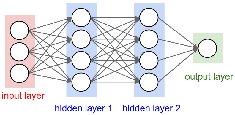
Multiple artificial neurons can act on the same inputs,. This defines a layer. We can have more than one layer until we produce one or more outputs.

The example above shows a network with 3 inputs, two layers of neurons, each with 4 neurons, followed by one layer that produces a single value output.

This architecture can be used as a binary classifier.

Next Lecture

Introduce and visualize our compute graph
Implement Backpropagation
Build out our neural network
Train and evaluate it

Recap

We introduced gradient descent for linear regression
We visualized the loss surface for linear regression
We saw how divergence can occur if the step size is too large
We defined an artificial neuron and a multi-layer perceptron

Introduction

The “Unreasonable” Effectiveness of Deep Neural Networks

Emergent Behavior in Pre-Trained Large Language Models

Theory Sometimes Follows Invention

Loss Functions for Model Fitting

Gradient Descent Intuitively

Derivatives on Single Variable Functions

Slope of a Function

Slope Shows the Influence of x on f

Interpretation of Slope

The Gradient

Gradient Descent on a Linear Regression Model

Example: Linear Regression

Challenges in Gradient Descent

Learning Rate

Complex Loss Surfaces

Recap

Neuron and Neural Networks

Artificial Neuron

Multi-Layer Perceptron (MLP) or Fully Connected Network (FCN)

Next Lecture

Recap

Slope Shows the Influence of $x$ on $f$