Code
import numpy as np
import scipy as sp
import matplotlib.pyplot as plt
import pandas as pd
import sklearn.datasets as sk_data
from sklearn.cluster import KMeans

import seaborn as sns![]()
import numpy as np
import scipy as sp
import matplotlib.pyplot as plt
import pandas as pd
import sklearn.datasets as sk_data
from sklearn.cluster import KMeans
import seaborn as snsHow many clusters would you say there are here?
X_rand, y_rand = sk_data.make_blobs(
    n_samples=[100, 100, 250, 70, 75, 80],
    centers = [[1, 2], [1.5, 1], [3, 2], [1.75, 3.25], [2, 4], [2.25, 3.25]],
    n_features = 2,
    center_box = (-10.0, 10.0),
    cluster_std = [.2, .2, .3, .1, .15, .15],
    random_state = 0
)
df_rand = pd.DataFrame(np.column_stack([X_rand[:, 0], X_rand[:, 1], y_rand]), columns = ['X', 'Y', 'label'])
df_rand = df_rand.astype({'label': 'int'})
df_rand['label3'] = [{0: 0, 1: 0, 2: 1, 3: 2, 4: 2, 5: 2}[x] for x in df_rand['label']]
df_rand['label4'] = [{0: 0, 1: 1, 2: 2, 3: 3, 4: 3, 5: 3}[x] for x in df_rand['label']]
df_rand['label5'] = [{0: 0, 1: 1, 2: 2, 3: 3, 4: 4, 5: 3}[x] for x in df_rand['label']]

# kmeans = KMeans(init = 'k-means++', n_clusters = 3, n_init = 100)
# df_rand['label'] = kmeans.fit_predict(df_rand[['X', 'Y']])

df_rand.plot('X', 'Y', kind = 'scatter',
                   colorbar = False, figsize = (6, 6))
plt.axis('square')
plt.axis('off')
plt.show()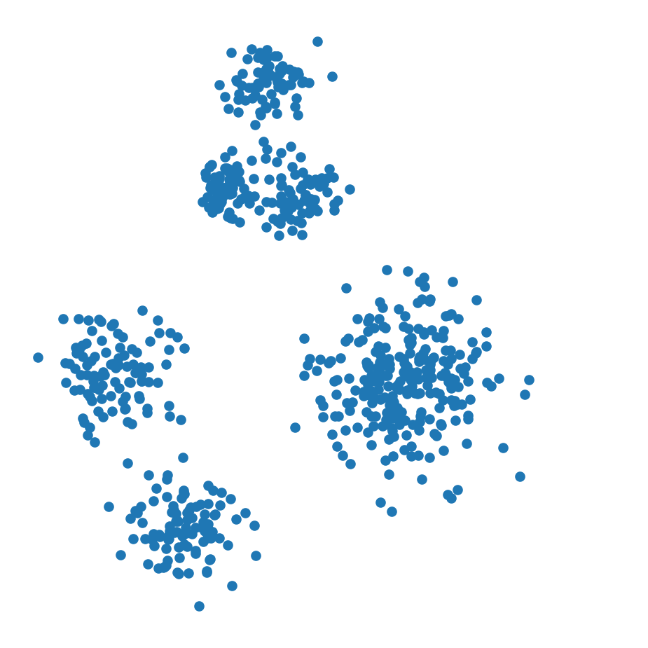
df_rand.plot('X', 'Y', kind = 'scatter', c = 'label3', colormap='viridis',
                   colorbar = False, figsize = (6, 6))
plt.axis('square')
plt.axis('off')
plt.show()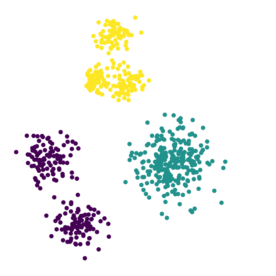
df_rand.plot('X', 'Y', kind = 'scatter', c = 'label4', colormap='viridis',
                   colorbar = False, figsize = (6, 6))
plt.axis('square')
plt.axis('off')
plt.show()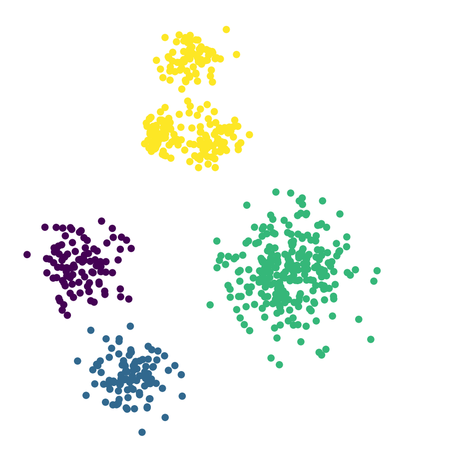
df_rand.plot('X', 'Y', kind = 'scatter', c = 'label5', colormap='viridis',
                   colorbar = False, figsize = (6, 6))
plt.axis('square')
plt.axis('off')
plt.show()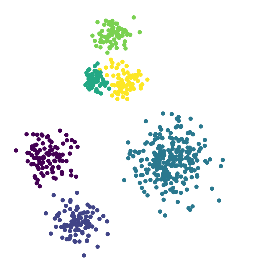
df_rand.plot('X', 'Y', kind = 'scatter', c = 'label', colormap='viridis',
                   colorbar = False, figsize = (6, 6))
plt.axis('square')
plt.axis('off')
plt.show()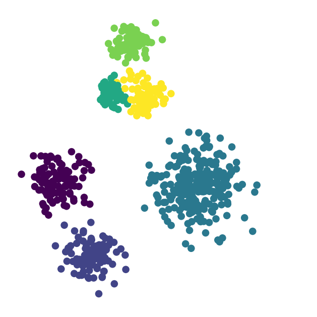
df_rand.plot('X', 'Y', kind = 'scatter', c = 'label', colormap='viridis',
                   colorbar = False, figsize = (4, 4))
plt.axis('square')
plt.axis('off')
plt.show()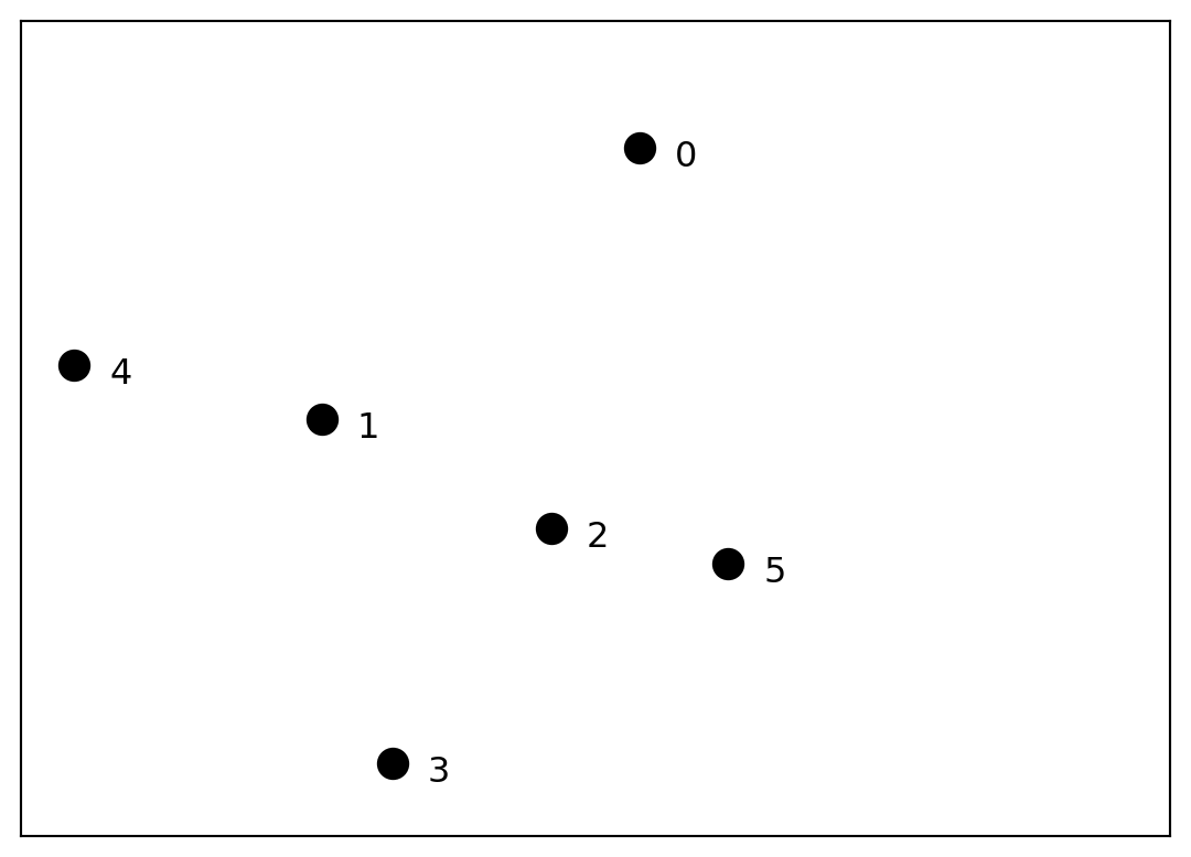
This dataset shows clustering on multiple scales.
To fully capture the structure in this dataset, two things are needed:
These observations motivate the notion of hierarchical clustering.
In hierarchical clustering, we move away from the partition notion of \(k\)-means,
and instead capture a more complex arrangement that includes containment of one cluster within another.
Note: GMMs relax the partitioning notion further!
Inspired by Hastie & Tibshirani lecture.
import matplotlib.pyplot as plt
import numpy as np

# Create 5 points with labels
points = {
    'A': (1.2, 5.2),
    'B': (2.7, 4.2),
    'C': (2, 6),
    'D': (5, 3),
    'E': (4, 2)
}

# Create the scatter plot
plt.figure(figsize=(6, 6))
for label, (x, y) in points.items():
    plt.scatter(x, y, s=100, alpha=0.7)
    plt.annotate(label, (x, y), xytext=(5, 5), textcoords='offset points',
                fontsize=12, fontweight='bold')

plt.xlabel('Feature 1')
plt.ylabel('Feature 2')
plt.title('2D Scatter Plot with 5 Labeled Points')
plt.grid(True, alpha=0.3)
plt.xlim(0, 7)
plt.ylim(0, 7)
plt.show()
import matplotlib.pyplot as plt
import numpy as np
from matplotlib.patches import Ellipse

# Create 5 points with labels (same as before)
points = {
    'A': (1.2, 5.2),
    'B': (2.7, 4.2),
    'C': (2, 6),
    'D': (5, 3),
    'E': (4, 2)
}

# Create the scatter plot
plt.figure(figsize=(6, 6))
for label, (x, y) in points.items():
    plt.scatter(x, y, s=100, alpha=0.7)
    plt.annotate(label, (x, y), xytext=(5, 5), textcoords='offset points',
                fontsize=12, fontweight='bold')

# Draw an ellipse around points A and C where A and C are the foci
A_x, A_y = points['A']
C_x, C_y = points['C']

# Calculate the distance between foci (A and C)
focal_distance = np.sqrt((C_x - A_x)**2 + (C_y - A_y)**2)

# Calculate center of ellipse (midpoint between foci)
center_x = (A_x + C_x) / 2
center_y = (A_y + C_y) / 2

# Calculate the angle of the major axis
angle = np.degrees(np.arctan2(C_y - A_y, C_x - A_x))

# Set semi-major axis (a) and semi-minor axis (b)
# For an ellipse: c = sqrt(a^2 - b^2) where c is half the focal distance
# We'll set a = focal_distance/2 + padding, then calculate b
a = focal_distance/2 + 0.4  # semi-major axis with padding
c = focal_distance/2  # half the focal distance
b = np.sqrt(a**2 - c**2)  # semi-minor axis

# Create and add the ellipse
ellipse = Ellipse((center_x, center_y), 2*a, 2*b, angle=angle,
                  facecolor='none', edgecolor='red', linewidth=2, linestyle='--')
plt.gca().add_patch(ellipse)

plt.xlabel('Feature 1')
plt.ylabel('Feature 2')
plt.title('2D Scatter Plot - First Cluster (A & C)')
plt.grid(True, alpha=0.3)
plt.xlim(0, 7)
plt.ylim(0, 7)
plt.show()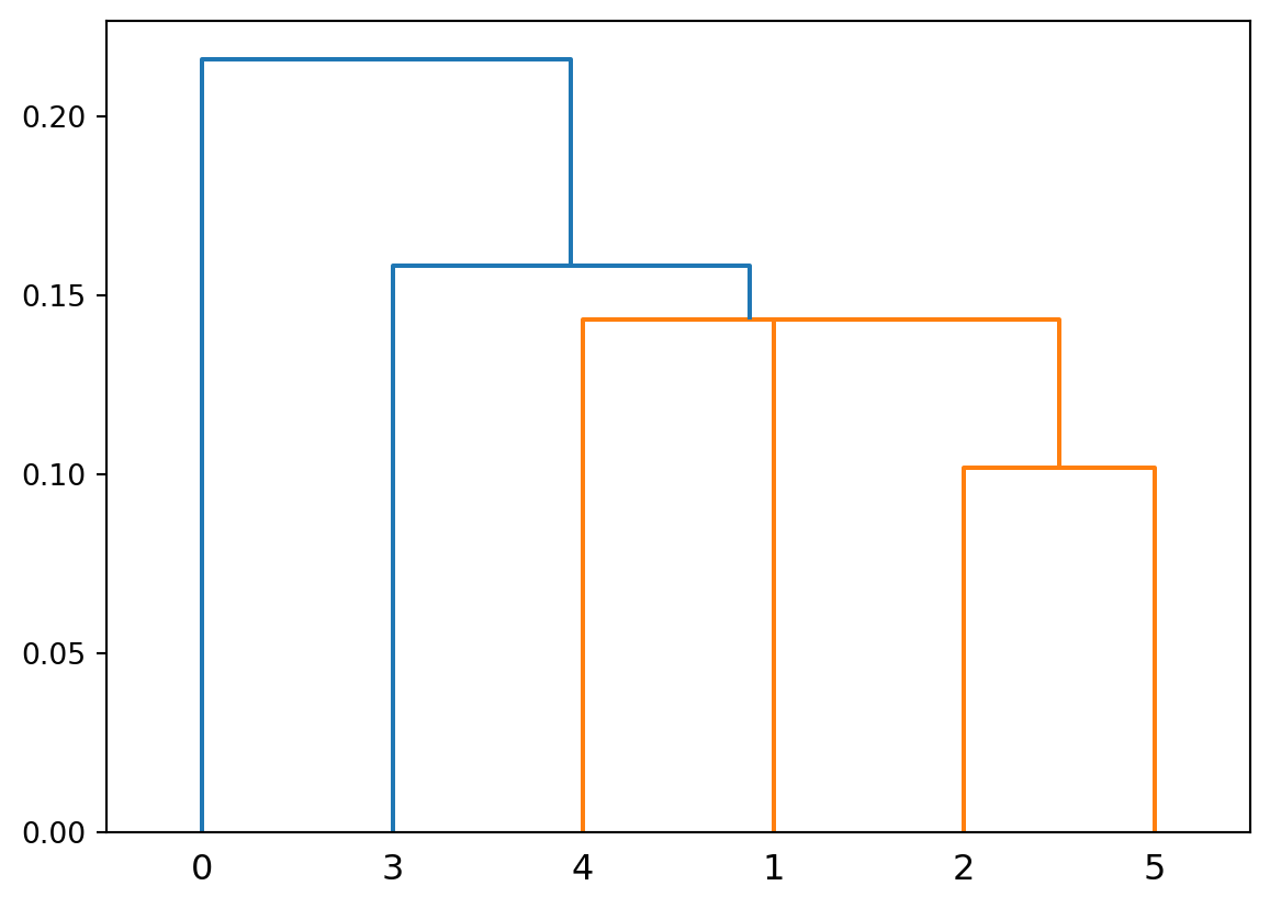
import matplotlib.pyplot as plt
import numpy as np
from matplotlib.patches import Ellipse

# Create 5 points with labels (same as before)
points = {
    'A': (1.2, 5.2),
    'B': (2.7, 4.2),
    'C': (2, 6),
    'D': (5, 3),
    'E': (4, 2)
}

# Create the scatter plot
plt.figure(figsize=(6, 6))
for label, (x, y) in points.items():
    plt.scatter(x, y, s=100, alpha=0.7)
    plt.annotate(label, (x, y), xytext=(5, 5), textcoords='offset points',
                fontsize=12, fontweight='bold')

# Draw an ellipse around points A and C where A and C are the foci
A_x, A_y = points['A']
C_x, C_y = points['C']

# Calculate the distance between foci (A and C)
focal_distance = np.sqrt((C_x - A_x)**2 + (C_y - A_y)**2)

# Calculate center of ellipse (midpoint between foci)
center_x = (A_x + C_x) / 2
center_y = (A_y + C_y) / 2

# Calculate the angle of the major axis
angle = np.degrees(np.arctan2(C_y - A_y, C_x - A_x))

# Set semi-major axis (a) and semi-minor axis (b)
# For an ellipse: c = sqrt(a^2 - b^2) where c is half the focal distance
# We'll set a = focal_distance/2 + padding, then calculate b
a = focal_distance/2 + 0.4  # semi-major axis with padding
c = focal_distance/2  # half the focal distance
b = np.sqrt(a**2 - c**2)  # semi-minor axis

# Create and add the ellipse for A and C
ellipse1 = Ellipse((center_x, center_y), 2*a, 2*b, angle=angle,
                   facecolor='none', edgecolor='red', linewidth=2, linestyle='--')
plt.gca().add_patch(ellipse1)

# Draw an ellipse around points E and D where E and D are the foci
E_x, E_y = points['E']
D_x, D_y = points['D']

# Calculate the distance between foci (E and D)
focal_distance_ED = np.sqrt((D_x - E_x)**2 + (D_y - E_y)**2)

# Calculate center of ellipse (midpoint between foci)
center_x_ED = (E_x + D_x) / 2
center_y_ED = (E_y + D_y) / 2

# Calculate the angle of the major axis
angle_ED = np.degrees(np.arctan2(D_y - E_y, D_x - E_x))

# Set semi-major axis (a) and semi-minor axis (b)
a_ED = focal_distance_ED/2 + 0.4  # semi-major axis with padding
c_ED = focal_distance_ED/2  # half the focal distance
b_ED = np.sqrt(a_ED**2 - c_ED**2)  # semi-minor axis

# Create and add the ellipse for E and D
ellipse2 = Ellipse((center_x_ED, center_y_ED), 2*a_ED, 2*b_ED, angle=angle_ED,
                   facecolor='none', edgecolor='blue', linewidth=2, linestyle='--')
plt.gca().add_patch(ellipse2)

plt.xlabel('Feature 1')
plt.ylabel('Feature 2')
plt.title('2D Scatter Plot - Two Clusters (A&C, E&D)')
plt.grid(True, alpha=0.3)
plt.xlim(0, 7)
plt.ylim(0, 7)
plt.show()
import matplotlib.pyplot as plt
import numpy as np
from matplotlib.patches import Ellipse

# Create 5 points with labels (same as before)
points = {
    'A': (1.2, 5.2),
    'B': (2.7, 4.2),
    'C': (2, 6),
    'D': (5, 3),
    'E': (4, 2)
}

# Create the scatter plot
plt.figure(figsize=(6, 6))
for label, (x, y) in points.items():
    plt.scatter(x, y, s=100, alpha=0.7)
    plt.annotate(label, (x, y), xytext=(5, 5), textcoords='offset points',
                fontsize=12, fontweight='bold')

# Draw an ellipse around points A and C where A and C are the foci
A_x, A_y = points['A']
C_x, C_y = points['C']

# Calculate the distance between foci (A and C)
focal_distance = np.sqrt((C_x - A_x)**2 + (C_y - A_y)**2)

# Calculate center of ellipse (midpoint between foci)
center_x = (A_x + C_x) / 2
center_y = (A_y + C_y) / 2

# Calculate the angle of the major axis
angle = np.degrees(np.arctan2(C_y - A_y, C_x - A_x))

# Set semi-major axis (a) and semi-minor axis (b)
# For an ellipse: c = sqrt(a^2 - b^2) where c is half the focal distance
# We'll set a = focal_distance/2 + padding, then calculate b
a = focal_distance/2 + 0.4  # semi-major axis with padding
c = focal_distance/2  # half the focal distance
b = np.sqrt(a**2 - c**2)  # semi-minor axis

# Create and add the ellipse for A and C
ellipse1 = Ellipse((center_x, center_y), 2*a, 2*b, angle=angle,
                   facecolor='none', edgecolor='red', linewidth=2, linestyle='--')
plt.gca().add_patch(ellipse1)

# Draw an ellipse around points E and D where E and D are the foci
E_x, E_y = points['E']
D_x, D_y = points['D']

# Calculate the distance between foci (E and D)
focal_distance_ED = np.sqrt((D_x - E_x)**2 + (D_y - E_y)**2)

# Calculate center of ellipse (midpoint between foci)
center_x_ED = (E_x + D_x) / 2
center_y_ED = (E_y + D_y) / 2

# Calculate the angle of the major axis
angle_ED = np.degrees(np.arctan2(D_y - E_y, D_x - E_x))

# Set semi-major axis (a) and semi-minor axis (b)
a_ED = focal_distance_ED/2 + 0.4  # semi-major axis with padding
c_ED = focal_distance_ED/2  # half the focal distance
b_ED = np.sqrt(a_ED**2 - c_ED**2)  # semi-minor axis

# Create and add the ellipse for E and D
ellipse2 = Ellipse((center_x_ED, center_y_ED), 2*a_ED, 2*b_ED, angle=angle_ED,
                   facecolor='none', edgecolor='blue', linewidth=2, linestyle='--')
plt.gca().add_patch(ellipse2)

# Draw a circle around points A, B, and C
A_x, A_y = points['A']
B_x, B_y = points['B']
C_x, C_y = points['C']

# Calculate the center of the circle (centroid of the three points)
center_x_ABC = (A_x + B_x + C_x) / 3
center_y_ABC = (A_y + B_y + C_y) / 3

# Calculate the radius as the maximum distance from center to any of the three points
dist_A = np.sqrt((A_x - center_x_ABC)**2 + (A_y - center_y_ABC)**2)
dist_B = np.sqrt((B_x - center_x_ABC)**2 + (B_y - center_y_ABC)**2)
dist_C = np.sqrt((C_x - center_x_ABC)**2 + (C_y - center_y_ABC)**2)
radius_ABC = max(dist_A, dist_B, dist_C) + 0.3  # Add some padding

# Create and add the circle
circle = plt.Circle((center_x_ABC, center_y_ABC), radius_ABC,
                   facecolor='none', edgecolor='green', linewidth=2, linestyle='--')
plt.gca().add_patch(circle)

plt.xlabel('Feature 1')
plt.ylabel('Feature 2')
plt.title('2D Scatter Plot - Three Clusters')
plt.grid(True, alpha=0.3)
plt.xlim(0, 7)
plt.ylim(0, 7)
plt.show()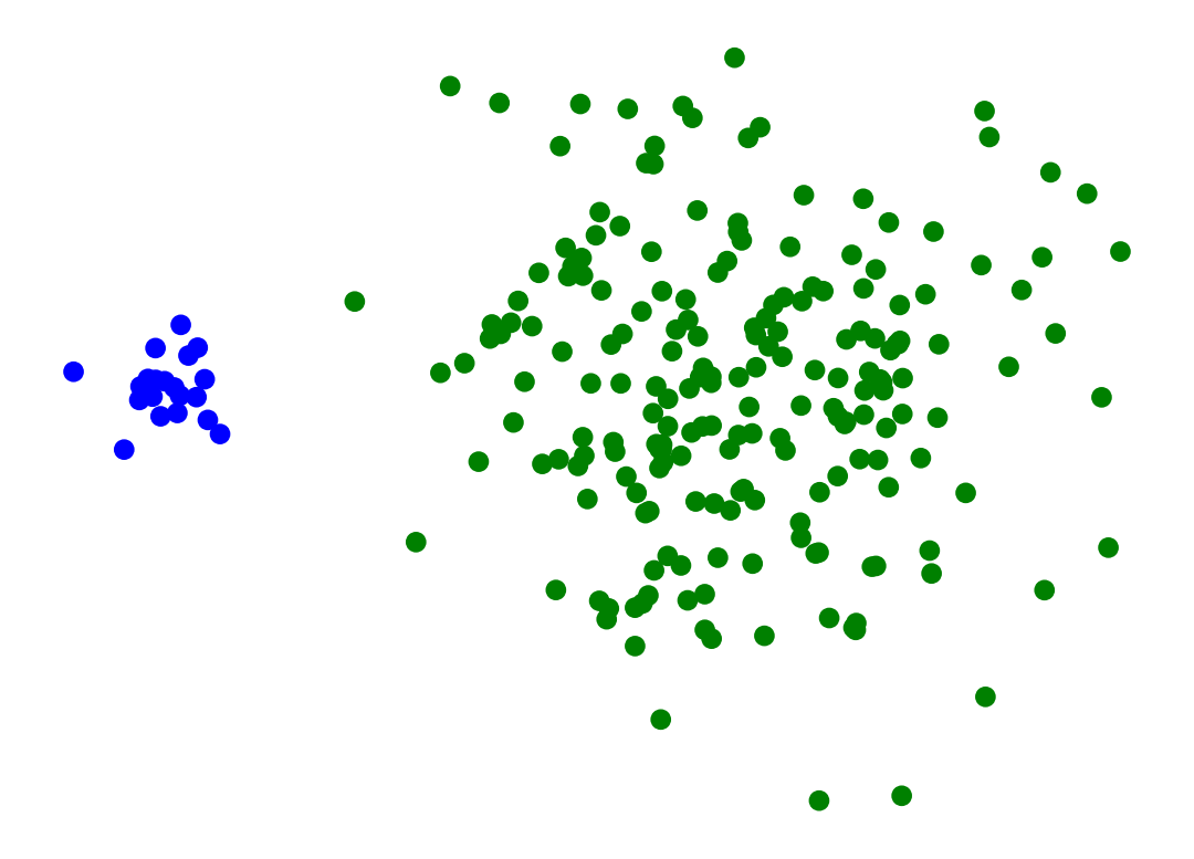
import matplotlib.pyplot as plt
import numpy as np
from matplotlib.patches import Ellipse

# Create 5 points with labels (same as before)
points = {
    'A': (1.2, 5.2),
    'B': (2.7, 4.2),
    'C': (2, 6),
    'D': (5, 3),
    'E': (4, 2)
}

# Create the scatter plot
plt.figure(figsize=(6, 6))
for label, (x, y) in points.items():
    plt.scatter(x, y, s=100, alpha=0.7)
    plt.annotate(label, (x, y), xytext=(5, 5), textcoords='offset points',
                fontsize=12, fontweight='bold')

# Draw an ellipse around points A and C where A and C are the foci
A_x, A_y = points['A']
C_x, C_y = points['C']

# Calculate the distance between foci (A and C)
focal_distance = np.sqrt((C_x - A_x)**2 + (C_y - A_y)**2)

# Calculate center of ellipse (midpoint between foci)
center_x = (A_x + C_x) / 2
center_y = (A_y + C_y) / 2

# Calculate the angle of the major axis
angle = np.degrees(np.arctan2(C_y - A_y, C_x - A_x))

# Set semi-major axis (a) and semi-minor axis (b)
# For an ellipse: c = sqrt(a^2 - b^2) where c is half the focal distance
# We'll set a = focal_distance/2 + padding, then calculate b
a = focal_distance/2 + 0.4  # semi-major axis with padding
c = focal_distance/2  # half the focal distance
b = np.sqrt(a**2 - c**2)  # semi-minor axis

# Create and add the ellipse for A and C
ellipse1 = Ellipse((center_x, center_y), 2*a, 2*b, angle=angle,
                   facecolor='none', edgecolor='red', linewidth=2, linestyle='--')
plt.gca().add_patch(ellipse1)

# Draw an ellipse around points E and D where E and D are the foci
E_x, E_y = points['E']
D_x, D_y = points['D']

# Calculate the distance between foci (E and D)
focal_distance_ED = np.sqrt((D_x - E_x)**2 + (D_y - E_y)**2)

# Calculate center of ellipse (midpoint between foci)
center_x_ED = (E_x + D_x) / 2
center_y_ED = (E_y + D_y) / 2

# Calculate the angle of the major axis
angle_ED = np.degrees(np.arctan2(D_y - E_y, D_x - E_x))

# Set semi-major axis (a) and semi-minor axis (b)
a_ED = focal_distance_ED/2 + 0.4  # semi-major axis with padding
c_ED = focal_distance_ED/2  # half the focal distance
b_ED = np.sqrt(a_ED**2 - c_ED**2)  # semi-minor axis

# Create and add the ellipse for E and D
ellipse2 = Ellipse((center_x_ED, center_y_ED), 2*a_ED, 2*b_ED, angle=angle_ED,
                   facecolor='none', edgecolor='blue', linewidth=2, linestyle='--')
plt.gca().add_patch(ellipse2)

# Draw a circle around points A, B, and C
A_x, A_y = points['A']
B_x, B_y = points['B']
C_x, C_y = points['C']

# Calculate the center of the circle (centroid of the three points)
center_x_ABC = (A_x + B_x + C_x) / 3
center_y_ABC = (A_y + B_y + C_y) / 3

# Calculate the radius as the maximum distance from center to any of the three points
dist_A = np.sqrt((A_x - center_x_ABC)**2 + (A_y - center_y_ABC)**2)
dist_B = np.sqrt((B_x - center_x_ABC)**2 + (B_y - center_y_ABC)**2)
dist_C = np.sqrt((C_x - center_x_ABC)**2 + (C_y - center_y_ABC)**2)
radius_ABC = max(dist_A, dist_B, dist_C) + 0.3  # Add some padding

# Create and add the circle
circle = plt.Circle((center_x_ABC, center_y_ABC), radius_ABC,
                   facecolor='none', edgecolor='green', linewidth=2, linestyle='--')
plt.gca().add_patch(circle)

# Draw an ellipse around all 5 points
all_x = [points[label][0] for label in points.keys()]
all_y = [points[label][1] for label in points.keys()]

# Calculate center of ellipse (centroid of all points)
center_x_all = np.mean(all_x)
center_y_all = np.mean(all_y)


width_all, height_all = 3.2, 7
angle_all = 40

print(width_all, height_all, angle_all, center_x_all, center_y_all)

# Create and add the ellipse around all points
ellipse_all = Ellipse((center_x_all, center_y_all), width_all, height_all, angle=angle_all,
                     facecolor='none', edgecolor='purple', linewidth=3, linestyle='-')
plt.gca().add_patch(ellipse_all)

plt.xlabel('Feature 1')
plt.ylabel('Feature 2')
plt.title('2D Scatter Plot - Final Cluster (All Points)')
plt.grid(True, alpha=0.3)
plt.xlim(0, 7)
plt.ylim(0, 7)
plt.show()
3.2 7 40 2.98 4.08
import matplotlib.pyplot as plt
import numpy as np
from matplotlib.patches import Ellipse
from scipy.cluster.hierarchy import dendrogram, linkage
from scipy.spatial.distance import pdist

# Create 5 points with labels (same as before)
points = {
    'A': (1.2, 5.2),
    'B': (2.7, 4.2),
    'C': (2, 6),
    'D': (5, 3),
    'E': (4, 2)
}

# Create figure with two subplots
fig, (ax1, ax2) = plt.subplots(1, 2, figsize=(12, 6))

# First subplot: Scatter plot with clusters
for label, (x, y) in points.items():
    ax1.scatter(x, y, s=100, alpha=0.7)
    ax1.annotate(label, (x, y), xytext=(5, 5), textcoords='offset points',
                fontsize=12, fontweight='bold')

# Draw an ellipse around points A and C where A and C are the foci
A_x, A_y = points['A']
C_x, C_y = points['C']

# Calculate the distance between foci (A and C)
focal_distance = np.sqrt((C_x - A_x)**2 + (C_y - A_y)**2)

# Calculate center of ellipse (midpoint between foci)
center_x = (A_x + C_x) / 2
center_y = (A_y + C_y) / 2

# Calculate the angle of the major axis
angle = np.degrees(np.arctan2(C_y - A_y, C_x - A_x))

# Set semi-major axis (a) and semi-minor axis (b)
a = focal_distance/2 + 0.4  # semi-major axis with padding
c = focal_distance/2  # half the focal distance
b = np.sqrt(a**2 - c**2)  # semi-minor axis

# Create and add the ellipse for A and C
ellipse1 = Ellipse((center_x, center_y), 2*a, 2*b, angle=angle,
                   facecolor='none', edgecolor='red', linewidth=2, linestyle='--')
ax1.add_patch(ellipse1)

# Draw an ellipse around points E and D where E and D are the foci
E_x, E_y = points['E']
D_x, D_y = points['D']

# Calculate the distance between foci (E and D)
focal_distance_ED = np.sqrt((D_x - E_x)**2 + (D_y - E_y)**2)

# Calculate center of ellipse (midpoint between foci)
center_x_ED = (E_x + D_x) / 2
center_y_ED = (E_y + D_y) / 2

# Calculate the angle of the major axis
angle_ED = np.degrees(np.arctan2(D_y - E_y, D_x - E_x))

# Set semi-major axis (a) and semi-minor axis (b)
a_ED = focal_distance_ED/2 + 0.4  # semi-major axis with padding
c_ED = focal_distance_ED/2  # half the focal distance
b_ED = np.sqrt(a_ED**2 - c_ED**2)  # semi-minor axis

# Create and add the ellipse for E and D
ellipse2 = Ellipse((center_x_ED, center_y_ED), 2*a_ED, 2*b_ED, angle=angle_ED,
                   facecolor='none', edgecolor='blue', linewidth=2, linestyle='--')
ax1.add_patch(ellipse2)

# Draw a circle around points A, B, and C
A_x, A_y = points['A']
B_x, B_y = points['B']
C_x, C_y = points['C']

# Calculate the center of the circle (centroid of the three points)
center_x_ABC = (A_x + B_x + C_x) / 3
center_y_ABC = (A_y + B_y + C_y) / 3

# Calculate the radius as the maximum distance from center to any of the three points
dist_A = np.sqrt((A_x - center_x_ABC)**2 + (A_y - center_y_ABC)**2)
dist_B = np.sqrt((B_x - center_x_ABC)**2 + (B_y - center_y_ABC)**2)
dist_C = np.sqrt((C_x - center_x_ABC)**2 + (C_y - center_y_ABC)**2)
radius_ABC = max(dist_A, dist_B, dist_C) + 0.3  # Add some padding

# Create and add the circle
circle = plt.Circle((center_x_ABC, center_y_ABC), radius_ABC,
                   facecolor='none', edgecolor='green', linewidth=2, linestyle='--')
ax1.add_patch(circle)

# Draw an ellipse around all 5 points
all_x = [points[label][0] for label in points.keys()]
all_y = [points[label][1] for label in points.keys()]

# Calculate center of ellipse (centroid of all points)
center_x_all = np.mean(all_x)
center_y_all = np.mean(all_y)

width_all, height_all = 3.2, 7
angle_all = 40

# Create and add the ellipse around all points
ellipse_all = Ellipse((center_x_all, center_y_all), width_all, height_all, angle=angle_all,
                     facecolor='none', edgecolor='purple', linewidth=3, linestyle='-')
ax1.add_patch(ellipse_all)

ax1.set_xlabel('Feature 1')
ax1.set_ylabel('Feature 2')
ax1.set_title('Clusters at Different Levels')
ax1.grid(True, alpha=0.3)
ax1.set_xlim(0, 7)
ax1.set_ylim(0, 7)

# Second subplot: Dendrogram
# Prepare data for hierarchical clustering
points_array = np.array(list(points.values()))
point_labels = list(points.keys())

# Calculate linkage matrix
linkage_matrix = linkage(points_array, method='ward')

# Create dendrogram
dendrogram(linkage_matrix, labels=point_labels, ax=ax2,
          leaf_rotation=0, leaf_font_size=12)
ax2.set_title('Hierarchical Clustering Dendrogram')
ax2.set_xlabel('Points')
ax2.set_ylabel('Distance')

plt.tight_layout()
plt.show()
import matplotlib.pyplot as plt
import numpy as np
from matplotlib.patches import Ellipse
from scipy.cluster.hierarchy import dendrogram, linkage
from scipy.spatial.distance import pdist

# Create 5 points with labels (same as before)
points = {
    'A': (1.2, 5.2),
    'B': (2.7, 4.2),
    'C': (2, 6),
    'D': (5, 3),
    'E': (4, 2)
}

# Create figure with two subplots
fig, (ax1, ax2) = plt.subplots(1, 2, figsize=(6, 3))

# First subplot: Scatter plot with clusters
for label, (x, y) in points.items():
    ax1.scatter(x, y, s=100, alpha=0.7)
    ax1.annotate(label, (x, y), xytext=(5, 5), textcoords='offset points',
                fontsize=12, fontweight='bold')

# Draw an ellipse around points A and C where A and C are the foci
A_x, A_y = points['A']
C_x, C_y = points['C']

# Calculate the distance between foci (A and C)
focal_distance = np.sqrt((C_x - A_x)**2 + (C_y - A_y)**2)

# Calculate center of ellipse (midpoint between foci)
center_x = (A_x + C_x) / 2
center_y = (A_y + C_y) / 2

# Calculate the angle of the major axis
angle = np.degrees(np.arctan2(C_y - A_y, C_x - A_x))

# Set semi-major axis (a) and semi-minor axis (b)
a = focal_distance/2 + 0.4  # semi-major axis with padding
c = focal_distance/2  # half the focal distance
b = np.sqrt(a**2 - c**2)  # semi-minor axis

# Create and add the ellipse for A and C
ellipse1 = Ellipse((center_x, center_y), 2*a, 2*b, angle=angle,
                   facecolor='none', edgecolor='red', linewidth=2, linestyle='--')
ax1.add_patch(ellipse1)

# Draw an ellipse around points E and D where E and D are the foci
E_x, E_y = points['E']
D_x, D_y = points['D']

# Calculate the distance between foci (E and D)
focal_distance_ED = np.sqrt((D_x - E_x)**2 + (D_y - E_y)**2)

# Calculate center of ellipse (midpoint between foci)
center_x_ED = (E_x + D_x) / 2
center_y_ED = (E_y + D_y) / 2

# Calculate the angle of the major axis
angle_ED = np.degrees(np.arctan2(D_y - E_y, D_x - E_x))

# Set semi-major axis (a) and semi-minor axis (b)
a_ED = focal_distance_ED/2 + 0.4  # semi-major axis with padding
c_ED = focal_distance_ED/2  # half the focal distance
b_ED = np.sqrt(a_ED**2 - c_ED**2)  # semi-minor axis

# Create and add the ellipse for E and D
ellipse2 = Ellipse((center_x_ED, center_y_ED), 2*a_ED, 2*b_ED, angle=angle_ED,
                   facecolor='none', edgecolor='blue', linewidth=2, linestyle='--')
ax1.add_patch(ellipse2)

# Draw a circle around points A, B, and C
A_x, A_y = points['A']
B_x, B_y = points['B']
C_x, C_y = points['C']

# Calculate the center of the circle (centroid of the three points)
center_x_ABC = (A_x + B_x + C_x) / 3
center_y_ABC = (A_y + B_y + C_y) / 3

# Calculate the radius as the maximum distance from center to any of the three points
dist_A = np.sqrt((A_x - center_x_ABC)**2 + (A_y - center_y_ABC)**2)
dist_B = np.sqrt((B_x - center_x_ABC)**2 + (B_y - center_y_ABC)**2)
dist_C = np.sqrt((C_x - center_x_ABC)**2 + (C_y - center_y_ABC)**2)
radius_ABC = max(dist_A, dist_B, dist_C) + 0.3  # Add some padding

# Create and add the circle
circle = plt.Circle((center_x_ABC, center_y_ABC), radius_ABC,
                   facecolor='none', edgecolor='green', linewidth=2, linestyle='--')
ax1.add_patch(circle)

# Draw an ellipse around all 5 points
all_x = [points[label][0] for label in points.keys()]
all_y = [points[label][1] for label in points.keys()]

# Calculate center of ellipse (centroid of all points)
center_x_all = np.mean(all_x)
center_y_all = np.mean(all_y)

width_all, height_all = 3.2, 7
angle_all = 40

# Create and add the ellipse around all points
ellipse_all = Ellipse((center_x_all, center_y_all), width_all, height_all, angle=angle_all,
                     facecolor='none', edgecolor='purple', linewidth=3, linestyle='-')
ax1.add_patch(ellipse_all)

ax1.set_xlabel('Feature 1')
ax1.set_ylabel('Feature 2')
ax1.set_title('Clusters at Different Levels')
ax1.grid(True, alpha=0.3)
ax1.set_xlim(0, 7)
ax1.set_ylim(0, 7)

# Second subplot: Dendrogram
# Prepare data for hierarchical clustering
points_array = np.array(list(points.values()))
point_labels = list(points.keys())

# Calculate linkage matrix
linkage_matrix = linkage(points_array, method='ward')

# Create dendrogram
dendrogram(linkage_matrix, labels=point_labels, ax=ax2,
          leaf_rotation=0, leaf_font_size=12)
ax2.set_title('Hierarchical Clustering Dendrogram')
ax2.set_xlabel('Points')
ax2.set_ylabel('Distance')

plt.tight_layout()
plt.show()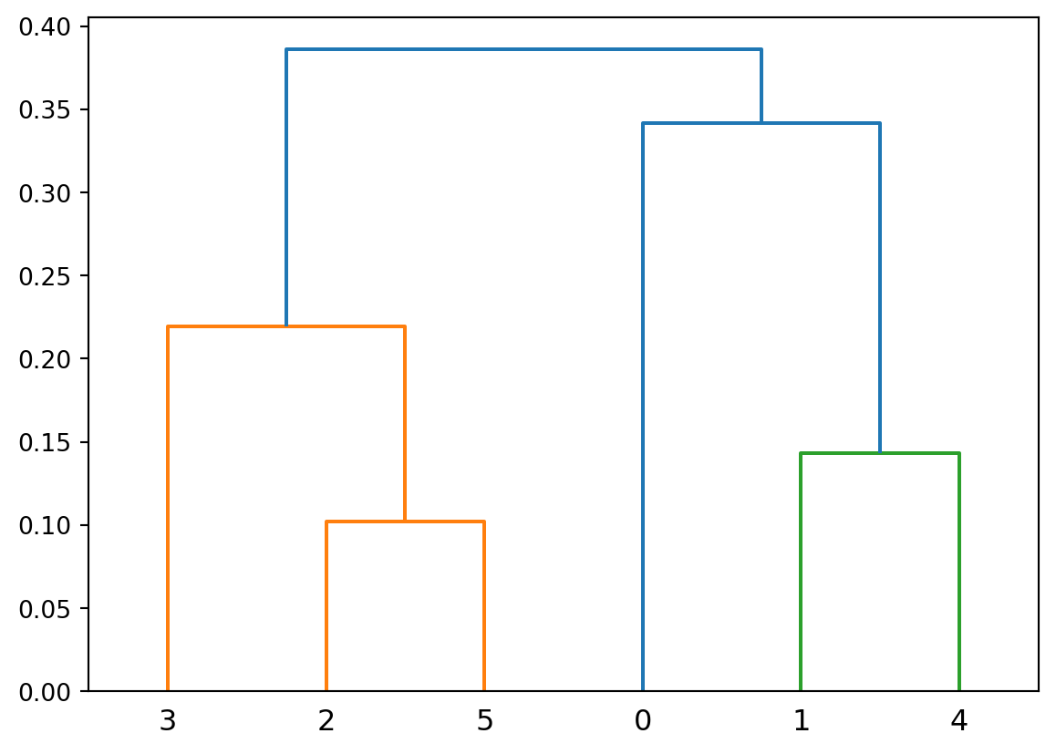
import matplotlib.pyplot as plt
import numpy as np
from matplotlib.patches import Ellipse
from scipy.cluster.hierarchy import dendrogram, linkage
from scipy.spatial.distance import pdist

# Create 5 points with labels (same as before)
points = {
    'A': (1.2, 5.2),
    'B': (2.7, 4.2),
    'C': (2, 6),
    'D': (5, 3),
    'E': (4, 2)
}

# Create figure with two subplots
fig, (ax1, ax2) = plt.subplots(1, 2, figsize=(6, 3))

# First subplot: Scatter plot with clusters
for label, (x, y) in points.items():
    ax1.scatter(x, y, s=100, alpha=0.7)
    ax1.annotate(label, (x, y), xytext=(5, 5), textcoords='offset points',
                fontsize=12, fontweight='bold')

# Draw an ellipse around points A and C where A and C are the foci
A_x, A_y = points['A']
C_x, C_y = points['C']

# Calculate the distance between foci (A and C)
focal_distance = np.sqrt((C_x - A_x)**2 + (C_y - A_y)**2)

# Calculate center of ellipse (midpoint between foci)
center_x = (A_x + C_x) / 2
center_y = (A_y + C_y) / 2

# Calculate the angle of the major axis
angle = np.degrees(np.arctan2(C_y - A_y, C_x - A_x))

# Set semi-major axis (a) and semi-minor axis (b)
a = focal_distance/2 + 0.4  # semi-major axis with padding
c = focal_distance/2  # half the focal distance
b = np.sqrt(a**2 - c**2)  # semi-minor axis

# Create and add the ellipse for A and C
ellipse1 = Ellipse((center_x, center_y), 2*a, 2*b, angle=angle,
                   facecolor='none', edgecolor='red', linewidth=2, linestyle='--')
ax1.add_patch(ellipse1)

# Draw an ellipse around points E and D where E and D are the foci
E_x, E_y = points['E']
D_x, D_y = points['D']

# Calculate the distance between foci (E and D)
focal_distance_ED = np.sqrt((D_x - E_x)**2 + (D_y - E_y)**2)

# Calculate center of ellipse (midpoint between foci)
center_x_ED = (E_x + D_x) / 2
center_y_ED = (E_y + D_y) / 2

# Calculate the angle of the major axis
angle_ED = np.degrees(np.arctan2(D_y - E_y, D_x - E_x))

# Set semi-major axis (a) and semi-minor axis (b)
a_ED = focal_distance_ED/2 + 0.4  # semi-major axis with padding
c_ED = focal_distance_ED/2  # half the focal distance
b_ED = np.sqrt(a_ED**2 - c_ED**2)  # semi-minor axis

# Create and add the ellipse for E and D
ellipse2 = Ellipse((center_x_ED, center_y_ED), 2*a_ED, 2*b_ED, angle=angle_ED,
                   facecolor='none', edgecolor='blue', linewidth=2, linestyle='--')
ax1.add_patch(ellipse2)

# Draw a circle around points A, B, and C
A_x, A_y = points['A']
B_x, B_y = points['B']
C_x, C_y = points['C']

# Calculate the center of the circle (centroid of the three points)
center_x_ABC = (A_x + B_x + C_x) / 3
center_y_ABC = (A_y + B_y + C_y) / 3

# Calculate the radius as the maximum distance from center to any of the three points
dist_A = np.sqrt((A_x - center_x_ABC)**2 + (A_y - center_y_ABC)**2)
dist_B = np.sqrt((B_x - center_x_ABC)**2 + (B_y - center_y_ABC)**2)
dist_C = np.sqrt((C_x - center_x_ABC)**2 + (C_y - center_y_ABC)**2)
radius_ABC = max(dist_A, dist_B, dist_C) + 0.3  # Add some padding

# Create and add the circle
circle = plt.Circle((center_x_ABC, center_y_ABC), radius_ABC,
                   facecolor='none', edgecolor='green', linewidth=2, linestyle='--')
ax1.add_patch(circle)

# Draw an ellipse around all 5 points
all_x = [points[label][0] for label in points.keys()]
all_y = [points[label][1] for label in points.keys()]

# Calculate center of ellipse (centroid of all points)
center_x_all = np.mean(all_x)
center_y_all = np.mean(all_y)

width_all, height_all = 3.2, 7
angle_all = 40

# Create and add the ellipse around all points
ellipse_all = Ellipse((center_x_all, center_y_all), width_all, height_all, angle=angle_all,
                     facecolor='none', edgecolor='purple', linewidth=3, linestyle='-')
ax1.add_patch(ellipse_all)

ax1.set_xlabel('Feature 1')
ax1.set_ylabel('Feature 2')
ax1.set_title('Clusters at Different Levels')
ax1.grid(True, alpha=0.3)
ax1.set_xlim(0, 7)
ax1.set_ylim(0, 7)

# Second subplot: Dendrogram
# Prepare data for hierarchical clustering
points_array = np.array(list(points.values()))
point_labels = list(points.keys())

# Calculate linkage matrix
linkage_matrix = linkage(points_array, method='ward')

# Create dendrogram
dendrogram(linkage_matrix, labels=point_labels, ax=ax2,
          leaf_rotation=0, leaf_font_size=12)
ax2.set_title('Dendrogram with Splits')
ax2.set_xlabel('Points')
ax2.set_ylabel('Distance')

# Add horizontal dashed red line at y=4 to show split level
ax2.axhline(y=4, color='red', linestyle='--', linewidth=2, alpha=0.8)

plt.tight_layout()

# Save the plot as a png image (uncomment to save)
# plt.savefig('figs/L08-dendrogram.png')
plt.show()
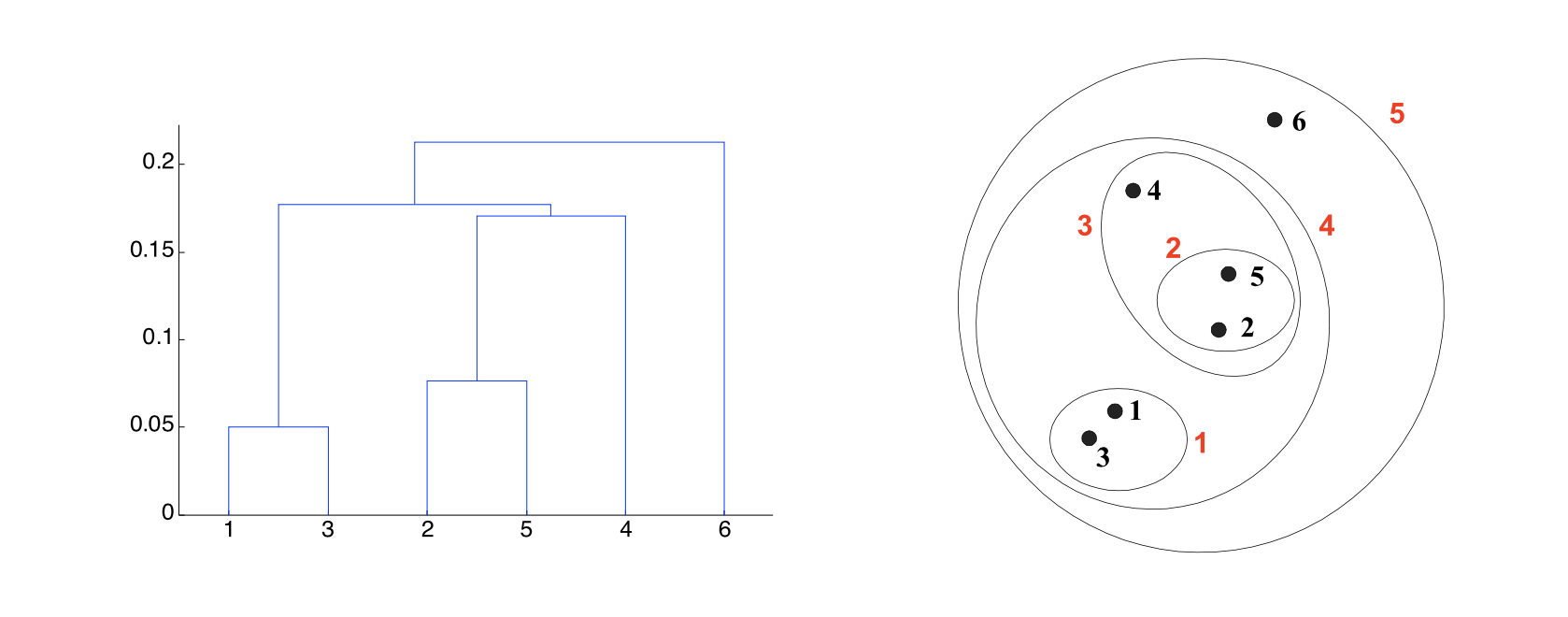
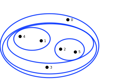
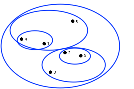
A hierarchical clustering produces a set of nested clusters organized into a tree.
A hierarchical clustering is visualized using a dendrogram
Hierarchical clustering has a number of advantages:
Another advantage is that the dendrogram may itself correspond to a meaningful structure, for example, a taxonomy.
Another aspect of hierachical clustering is that it can handle certain cases better than \(k\)-means.
Because of the nature of the \(k\)-means algorithm, \(k\)-means tends to produce:
In many real-world situations, clusters may not be round, they may be of unequal size, and they may overlap.
Hence we would like clustering algorithms that can work in those cases also.
Create a hierarchical cluster and dendogram for this data.
import matplotlib.pyplot as plt
import numpy as np
from matplotlib.patches import Ellipse
from scipy.cluster.hierarchy import dendrogram, linkage
from scipy.spatial.distance import pdist

# Create 5 points with labels (same as before)
points = {
    'A': (3.4, 6.1),
    'B': (1.8, 2.3),
    'C': (4.6, 4.9),
    'D': (1.6, 5.6),
    'E': (2.9, 1.7)
}

# Create figure with two subplots
fig, (ax1, ax2) = plt.subplots(1, 2, figsize=(10, 5))

# First subplot: Scatter plot with clusters
for label, (x, y) in points.items():
    ax1.scatter(x, y, s=100, alpha=0.7)
    ax1.annotate(label, (x, y), xytext=(5, 5), textcoords='offset points',
                fontsize=12, fontweight='bold')


ax1.set_xlabel('Feature 1')
ax1.set_ylabel('Feature 2')
ax1.set_title('Clusters at Different Levels')
ax1.grid(True, alpha=0.3)
ax1.set_xlim(0, 7)
ax1.set_ylim(0, 7)

# Create empty axis with 5 evenly spaced ticks
ax2.set_xlim(0, 4)
ax2.set_ylim(0, 1)
ax2.set_xticks([0, 1, 2, 3, 4])
ax2.set_xticklabels([])
ax2.set_yticks([0, 0.25, 0.5, 0.75, 1])
ax2.set_yticklabels([])
ax2.set_title('Dendogram')
ax2.set_xlabel('Points')
ax2.set_ylabel('Distance')

plt.tight_layout()

# Save the plot as a png image (uncomment to save)
# plt.savefig('figs/L08-dendrogram.png')
plt.show()
There are two main approaches to hierarchical clustering: “bottom-up” and “top-down.”
Agglomerative Clustering (“bottom-up”):
Divisive Clustering (“top-down”):
To illustrate the impact of the choice of cluster distances, we’ll focus on agglomerative clustering.
An \((n-1,4)\) shaped linkage matrix.
Where each row is [idx1, idx2, dist, sample_count] is a single step in the clustering process and
idx1 and idx2 are indices of the cluster being merged, where
And sample_count is the number of original data samples in the new cluster.
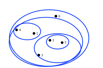
Let’s calculate and display the linkage matrix for our 5 data points A-E:
# Create 5 points with labels (same as before)
points = {
    'A': (1.2, 5.2),
    'B': (2.7, 4.2),
    'C': (2, 6),
    'D': (5, 3),
    'E': (4, 2)
}

# Prepare data for hierarchical clustering
points_array = np.array(list(points.values()))
point_labels = list(points.keys())

# Calculate linkage matrix using Ward's method
linkage_matrix = linkage(points_array, method='ward')

print("Linkage Matrix for 5 data points A-E:")
print("Format: [idx1, idx2, distance, sample_count]")
print("=" * 50)
print(linkage_matrix)
print("=" * 50)

# Display with labels for better understanding
print("\nInterpretation:")
print(f"Row 0: Merge points 0 and 2 (A and C) at distance {linkage_matrix[0,2]:.2f}")
print(f"Row 1: Merge points 3 and 4 (D and E) at distance {linkage_matrix[1,2]:.2f}")
print(f"Row 2: Merge point 1 (B) with cluster 5 (A&C) at distance {linkage_matrix[2,2]:.2f}")
print(f"Row 3: Merge cluster 6 (A&B&C) with cluster 7 (D&E) at distance {linkage_matrix[3,2]:.2f}")
Linkage Matrix for 5 data points A-E:
Format: [idx1, idx2, distance, sample_count]
==================================================
[[0. 2. 1.13137085 2. ]
[3. 4. 1.41421356 2. ]
[1. 5. 2.05588586 3. ]
[6. 7. 5.66085977 5. ]]
==================================================
Interpretation:
Row 0: Merge points 0 and 2 (A and C) at distance 1.13
Row 1: Merge points 3 and 4 (D and E) at distance 1.41
Row 2: Merge point 1 (B) with cluster 5 (A&C) at distance 2.06
Row 3: Merge cluster 6 (A&B&C) with cluster 7 (D&E) at distance 5.66
Given two clusters, how do we define the distance between them?
Here are three natural ways to do it.
Single-Linkage: the distance between two clusters is the distance between the closest two points that are in different clusters.
\[ D_\text{single}(i,j) = \min_{x, y}\{d(x, y) \,|\, x \in C_i, y \in C_j\} \]
Complete-Linkage: the distance between two clusters is the distance between the farthest two points that are in different clusters.
\[ D_\text{complete}(i,j) = \max_{x, y}\{d(x, y) \,|\, x \in C_i, y \in C_j\} \]
Average-Linkage: the distance between two clusters is the average distance between all pairs of points from different clusters.
\[ D_\text{average}(i,j) = \frac{1}{|C_i|\cdot|C_j|}\sum_{x \in C_i,\, y \in C_j}d(x, y) \]
Notice that it is easy to express the definitions above in terms of similarity instead of distance.
Here is a set of 6 points that we will cluster to show differences between distance metrics.
plt.figure(figsize=(6,4))
pt_x = [0.4, 0.22, 0.35, 0.26, 0.08, 0.45]
pt_y = [0.53, 0.38, 0.32, 0.19, 0.41, 0.30]
plt.plot(pt_x, pt_y, 'o', markersize = 10, color = 'k')
plt.ylim([.15, .60])
plt.xlim([0.05, 0.70])
for i in range(6):
    plt.annotate(f'{i}', (pt_x[i]+0.02, pt_y[i]-0.01), fontsize = 12)
plt.axis('on')
plt.xticks([])
plt.yticks([])
plt.show()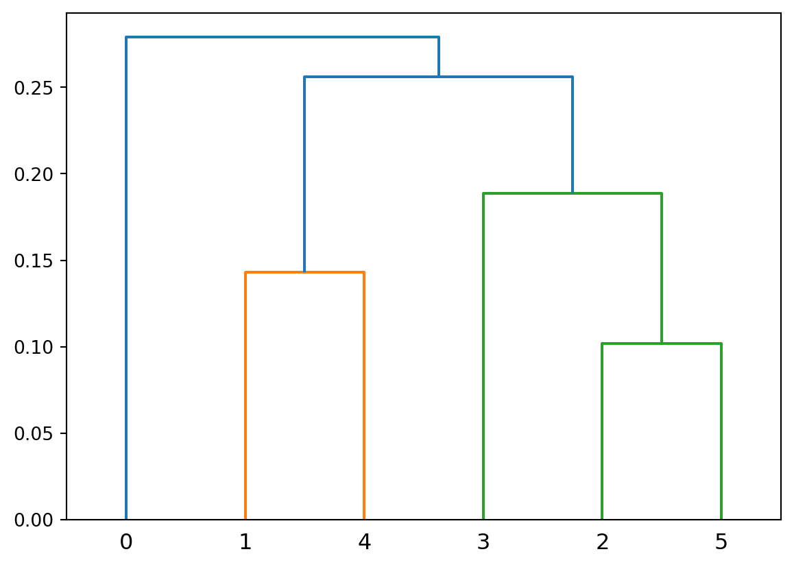
We can calculate the distance matrix
X = np.array([pt_x, pt_y]).T
from scipy.spatial import distance_matrix
labels = ['p0', 'p1', 'p2', 'p3', 'p4', 'p5']
D = pd.DataFrame(distance_matrix(X, X), index = labels, columns = labels)
D.style.format('{:.2f}')| p0 | p1 | p2 | p3 | p4 | p5 | |
|---|---|---|---|---|---|---|
| p0 | 0.00 | 0.23 | 0.22 | 0.37 | 0.34 | 0.24 |
| p1 | 0.23 | 0.00 | 0.14 | 0.19 | 0.14 | 0.24 |
| p2 | 0.22 | 0.14 | 0.00 | 0.16 | 0.28 | 0.10 |
| p3 | 0.37 | 0.19 | 0.16 | 0.00 | 0.28 | 0.22 |
| p4 | 0.34 | 0.14 | 0.28 | 0.28 | 0.00 | 0.39 |
| p5 | 0.24 | 0.24 | 0.10 | 0.22 | 0.39 | 0.00 |
import scipy.cluster
import scipy.cluster.hierarchy as hierarchy
Z = hierarchy.linkage(X, method='single', metric='euclidean')
hierarchy.dendrogram(Z)
plt.show()
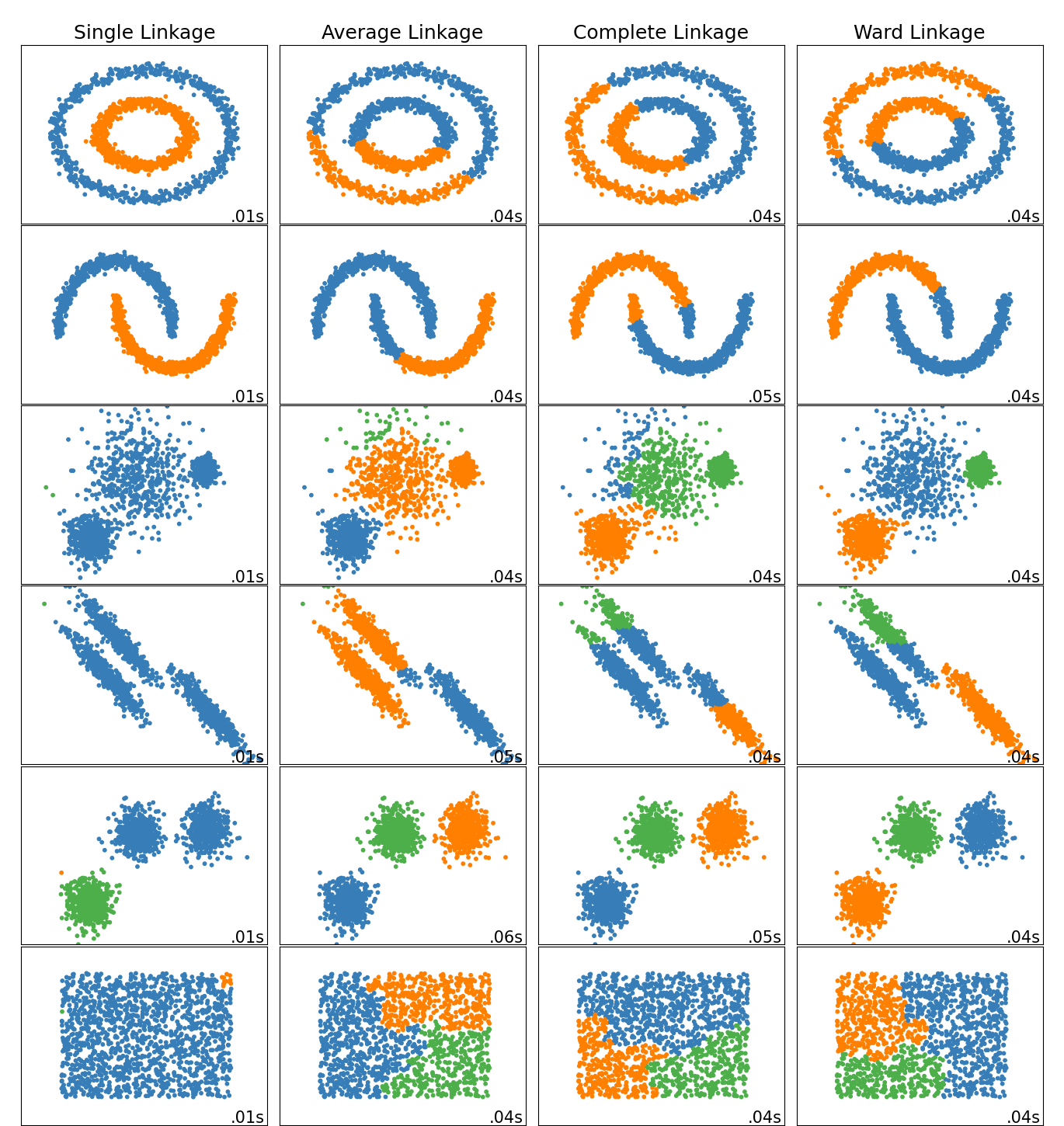
Single-linkage clustering can handle non-elliptical shapes.
Here we use SciPy’s fcluster to form flat custers from hierarchical clustering.
X_moon_05, y_moon_05 = sk_data.make_moons(random_state = 0, noise = 0.05)

Z = hierarchy.linkage(X_moon_05, method='single')
labels = hierarchy.fcluster(Z, 2, criterion = 'maxclust')

plt.scatter(X_moon_05[:, 0], X_moon_05[:, 1], c = [['b','g'][i-1] for i in labels])
plt.axis('off')
plt.show()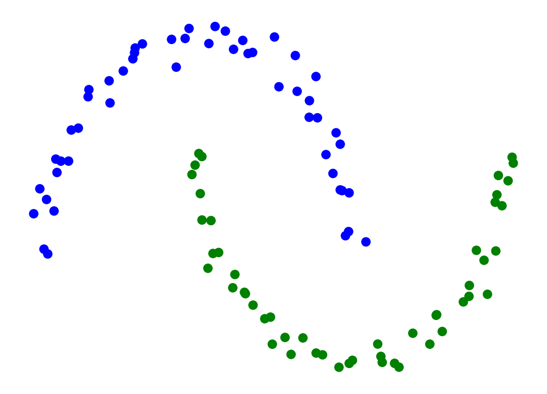
Single-Linkage can find different sized clusters:
X_rand_lo, y_rand_lo = sk_data.make_blobs(n_samples=[20, 200], centers = [[1, 1], [3, 1]], n_features = 2,
                          center_box = (-10.0, 10.0), cluster_std = [.1, .5], random_state = 0)

Z = hierarchy.linkage(X_rand_lo, method='single')
labels = hierarchy.fcluster(Z, 2, criterion = 'maxclust')

plt.scatter(X_rand_lo[:, 0], X_rand_lo[:, 1], c = [['b','g'][i-1] for i in labels])
# plt.title('Single-Linkage Can Find Different-Sized Clusters')
plt.axis('off')
plt.show()
Single-linkage clustering can be sensitive to noise and outliers.
The results can change drastically on even slightly more noisy data.
X_moon_10, y_moon_10 = sk_data.make_moons(random_state = 0, noise = 0.1)

Z = hierarchy.linkage(X_moon_10, method='single')
labels = hierarchy.fcluster(Z, 2, criterion = 'maxclust')

plt.scatter(X_moon_10[:, 0], X_moon_10[:, 1], c = [['b','g'][i-1] for i in labels])
# plt.title('Single-Linkage Clustering Changes Drastically on Slightly More Noisy Data')
plt.axis('off')
plt.show()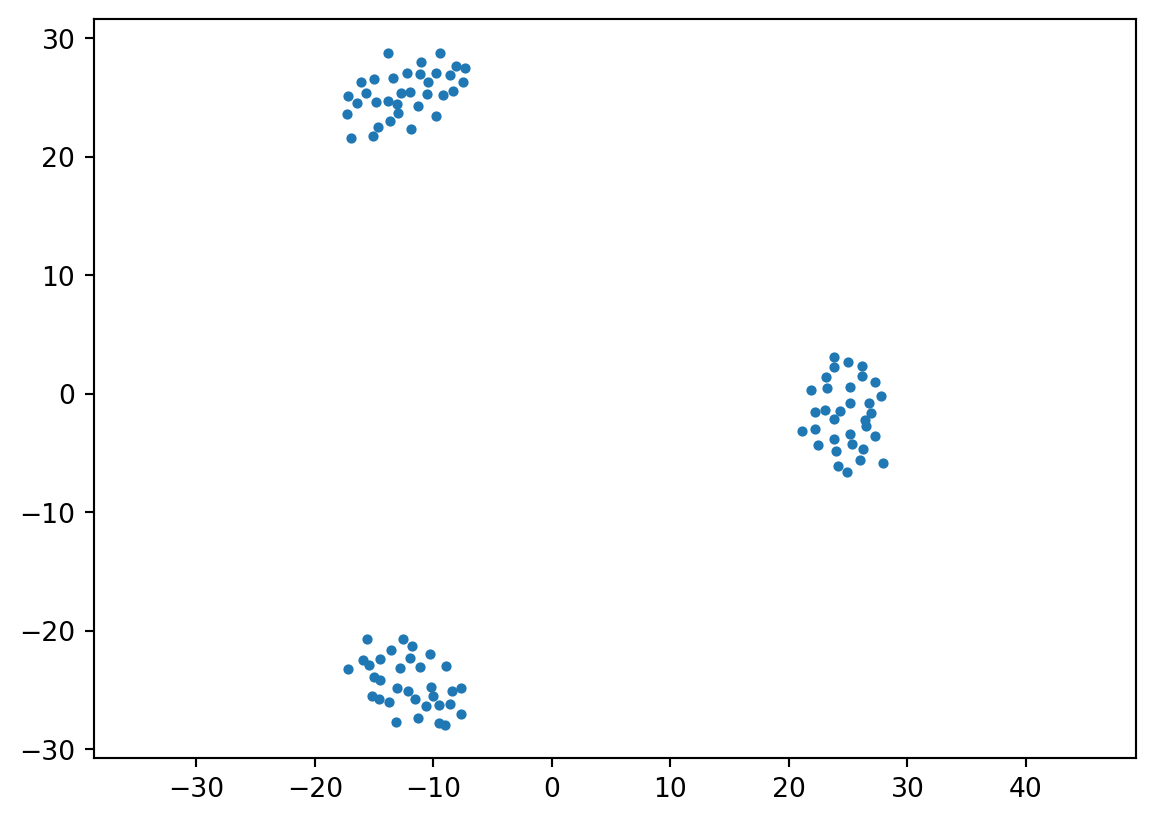
And here’s another example where we bump the standard deviation on the clusters slightly.
X_rand_hi, y_rand_hi = sk_data.make_blobs(n_samples=[20, 200], centers = [[1, 1], [3, 1]], n_features = 2,
                          center_box = (-10.0, 10.0), cluster_std = [.15, .6], random_state = 0)

Z = hierarchy.linkage(X_rand_hi, method='single')
labels = hierarchy.fcluster(Z, 2, criterion = 'maxclust')

plt.scatter(X_rand_hi[:, 0], X_rand_hi[:, 1], c = [['b','g'][i-1] for i in labels])
plt.axis('off')
plt.show()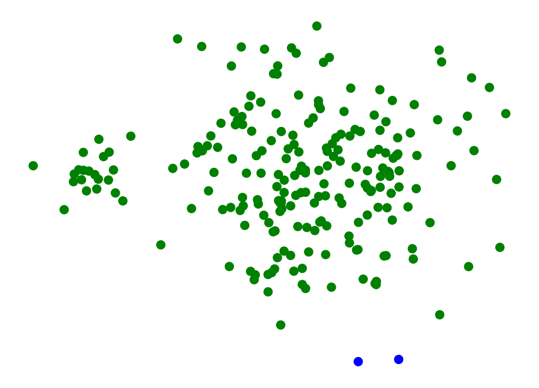
Z = hierarchy.linkage(X, method='complete')
hierarchy.dendrogram(Z)
plt.show()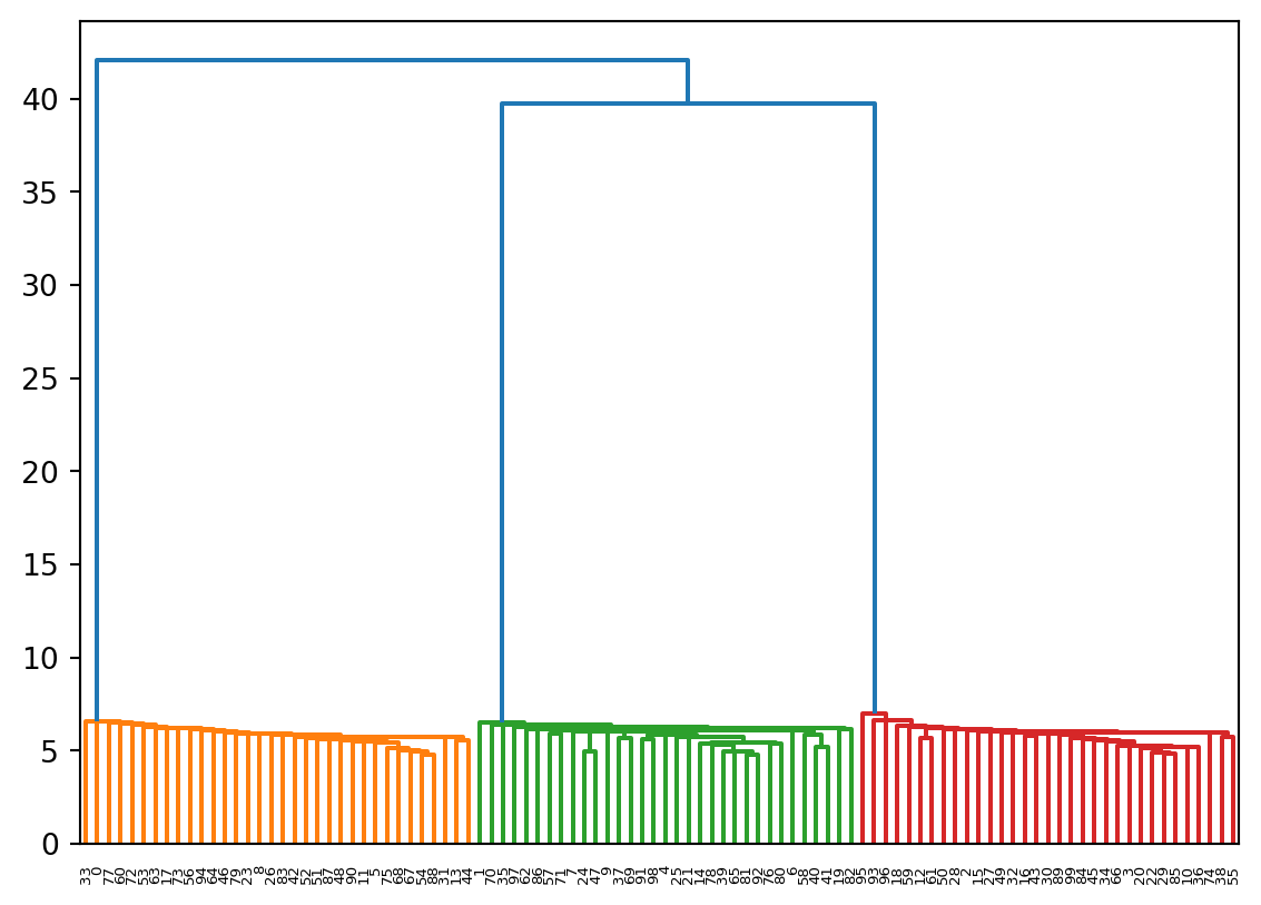
Produces more-balanced clusters – more-equal diameters
X_moon_05, y_moon_05 = sk_data.make_moons(random_state = 0, noise = 0.05)

Z = hierarchy.linkage(X_moon_05, method='complete')
labels = hierarchy.fcluster(Z, 2, criterion = 'maxclust')

plt.scatter(X_moon_05[:, 0], X_moon_05[:, 1], c = [['b','g'][i-1] for i in labels])
plt.axis('off')
plt.show()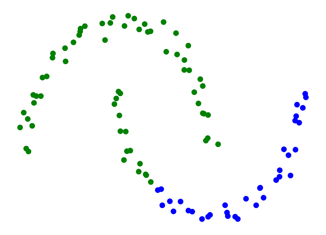
Z = hierarchy.linkage(X_rand_hi, method='complete')
labels = hierarchy.fcluster(Z, 2, criterion = 'maxclust')

plt.scatter(X_rand_hi[:, 0], X_rand_hi[:, 1], c = [['b','g'][i-1] for i in labels])
plt.axis('off')
plt.show()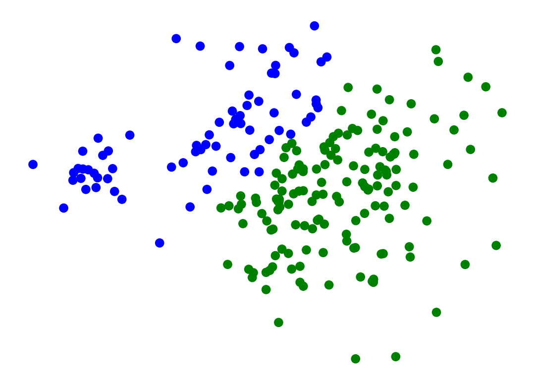
Less susceptible to noise:
Z = hierarchy.linkage(X_moon_10, method='complete')
labels = hierarchy.fcluster(Z, 2, criterion = 'maxclust')
plt.scatter(X_moon_10[:, 0], X_moon_10[:, 1], c = [['b','g'][i-1] for i in labels])

plt.axis('off')
plt.show()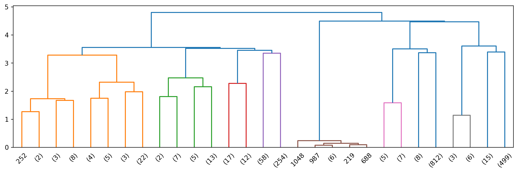
Some disadvantages for complete-linkage clustering are:
Z = hierarchy.linkage(X, method='average')
hierarchy.dendrogram(Z)
plt.show()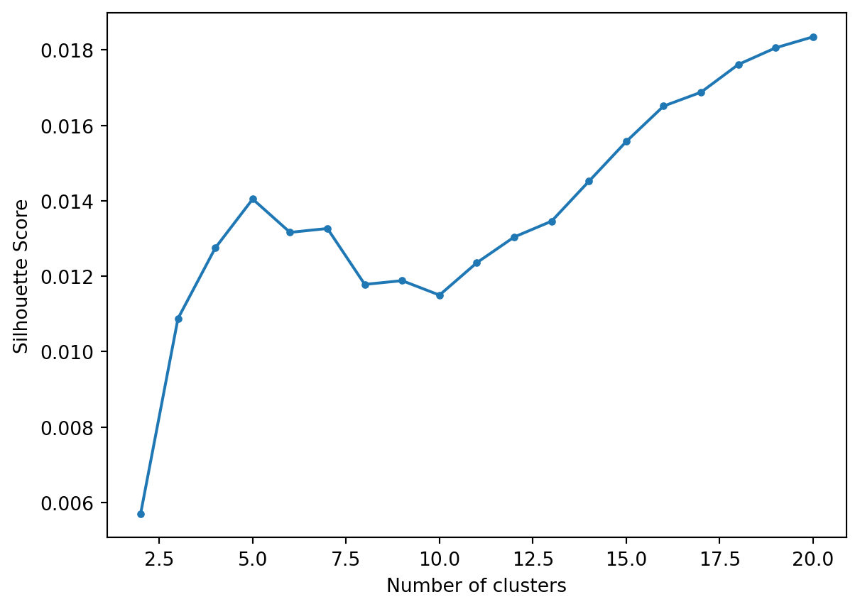
Average-Linkage clustering is in some sense a compromise between Single-linkage and Complete-linkage clustering.
Strengths:
Limitations:
Produces more isotropic clusters.
Z = hierarchy.linkage(X_moon_10, method='average')
labels = hierarchy.fcluster(Z, 2, criterion = 'maxclust')
plt.scatter(X_moon_10[:, 0], X_moon_10[:, 1], c = [['b','g'][i-1] for i in labels])

plt.axis('off')
plt.show()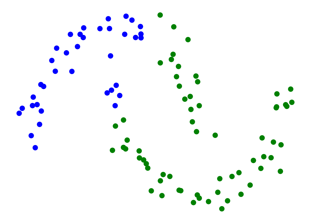
More resistant to noise than Single-Linkage.
Z = hierarchy.linkage(X_rand_hi, method='average')
labels = hierarchy.fcluster(Z, 2, criterion = 'maxclust')
plt.scatter(X_rand_hi[:, 0], X_rand_hi[:, 1], c = [['b','g'][i-1] for i in labels])

plt.axis('off')
plt.show()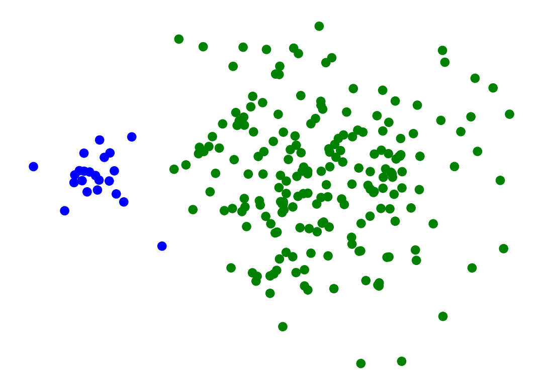
Finally, we consider one more cluster distance.
Ward’s distance asks “What if we combined these two clusters – how would clustering improve?”
To define “how would clustering improve?” we appeal to the \(k\)-means criterion.
So:
Ward’s Distance between clusters \(C_i\) and \(C_j\) is the difference between the total within cluster sum of squares for the two clusters separately, compared to the within cluster sum of squares resulting from merging the two clusters into a new cluster \(C_{i+j}\):
\[ D_\text{Ward}(i, j) = \sum_{x \in C_i} (x - c_i)^2 + \sum_{x \in C_j} (x - c_j)^2 - \sum_{x \in C_{i+j}} (x - c_{i+j})^2 \]
where \(c_i, c_j, c_{i+j}\) are the corresponding cluster centroids.
In a sense, this cluster distance results in a hierarchical analog of \(k\)-means.
As a result, it has properties similar to \(k\)-means:
Hence it tends to behave more like average-linkage hierarchical clustering.
Now we’ll look at doing hierarchical clustering in practice.
We’ll use 1/10th of the synthetic data set from the beginning of this lecture.
scipy has a comprehensive set of clustering tools.
X, y = sk_data.make_blobs(
    n_samples=[10, 10, 25, 7, 7, 8],
    centers = [[1, 2], [1.5, 1], [3, 2], [1.75, 3.25], [2, 4], [2.25, 3.25]],
    n_features = 2,
    center_box = (-10.0, 10.0),
    cluster_std = [.2, .2, .3, .1, .15, .15],
    random_state = 0
)

df_rand = pd.DataFrame(np.column_stack([X[:, 0], X[:, 1], y]), columns = ['X', 'Y', 'label'])

df_rand.plot('X', 'Y', kind = 'scatter',
                   colorbar = False, figsize = (5, 5))
plt.axis('square')
plt.axis('off')
plt.show()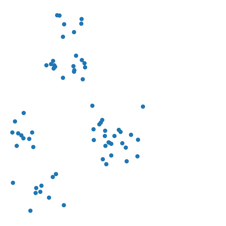
Let’s run hierarchical clustering on our synthetic dataset.
Try the other linkage methods and see how the clustering and dendrogram changes.
# linkages = ['single','complete','average','weighted','ward']
Z = hierarchy.linkage(X, method = 'single')
And draw the dendrogram.
R = hierarchy.dendrogram(Z)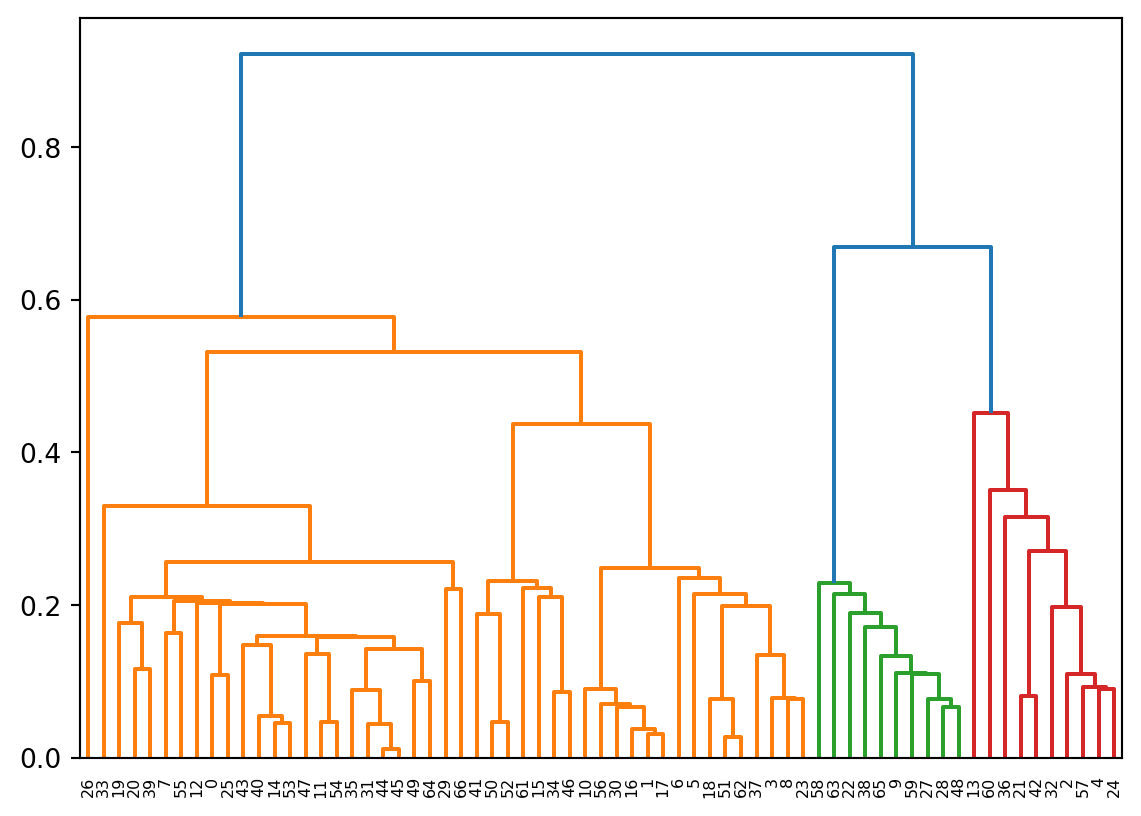
Once again we’ll use the “20 Newsgroup” data provided as example data in sklearn. Experiment with different metrics.
Load three of the newsgroups.
from sklearn.datasets import fetch_20newsgroups
categories = ['comp.os.ms-windows.misc', 'sci.space','rec.sport.baseball']
news_data = fetch_20newsgroups(subset = 'train', categories = categories)
Vectorize the data.
from sklearn.feature_extraction.text import TfidfVectorizer
vectorizer = TfidfVectorizer(stop_words='english', min_df = 4, max_df = 0.8)
data = vectorizer.fit_transform(news_data.data).todense()
data.shape
(1781, 9409)# linkages are one of 'single','complete','average','weighted','ward'
#
# metrics can be ‘braycurtis’, ‘canberra’, ‘chebyshev’, ‘cityblock’, ‘correlation’, ‘cosine’,
# ‘dice’, ‘euclidean’, ‘hamming’, ‘jaccard’, ‘kulsinski’, ‘mahalanobis’, ‘matching’,
# ‘minkowski’, ‘rogerstanimoto’, ‘russellrao’, ‘seuclidean’, ‘sokalmichener’, ‘sokalsneath’,
# ‘sqeuclidean’, ‘yule’.
Z_20ng = hierarchy.linkage(data, method = 'ward', metric = 'euclidean')
plt.figure(figsize=(14,4))
R_20ng = hierarchy.dendrogram(Z_20ng, p=4, truncate_mode = 'level', show_leaf_counts=True)
Let’s flatten the hierarchy to different numbers clusters and calculate the Silhouette Score.
import sklearn.metrics as metrics

max_clusters = 20
s = np.zeros(max_clusters+1)

for k in range(2, max_clusters+1):
    clusters = hierarchy.fcluster(Z_20ng, k, criterion = 'maxclust')
    s[k] = metrics.silhouette_score(np.asarray(data), clusters, metric = 'euclidean')

plt.plot(range(2, len(s)), s[2:], '.-')
plt.xlabel('Number of clusters')
plt.ylabel('Silhouette Score')
plt.show()
/Users/tgardos/Source/courses/ds701/DS701-Course-Notes/.venv/lib/python3.10/site-packages/sklearn/utils/extmath.py:203: RuntimeWarning: divide by zero encountered in matmul
ret = a @ b
/Users/tgardos/Source/courses/ds701/DS701-Course-Notes/.venv/lib/python3.10/site-packages/sklearn/utils/extmath.py:203: RuntimeWarning: overflow encountered in matmul
ret = a @ b
/Users/tgardos/Source/courses/ds701/DS701-Course-Notes/.venv/lib/python3.10/site-packages/sklearn/utils/extmath.py:203: RuntimeWarning: invalid value encountered in matmul
ret = a @ b
We see a first peak at 5.
Top terms per cluster when we flatten to a depth of 5.
k = 5
clusters = hierarchy.fcluster(Z_20ng, k, criterion = 'maxclust')
for i in range(1,k+1):
    items = np.array([item for item,clust in zip(data, clusters) if clust == i])
    centroids = np.squeeze(items).mean(axis = 0)
    asc_order_centroids = centroids.argsort()#[:, ::-1]
    order_centroids = asc_order_centroids[::-1]
    terms = vectorizer.get_feature_names_out()
    print(f'Cluster {i}:')
    for ind in order_centroids[:10]:
        print(f' {terms[ind]}')
    print('')
Cluster 1:
space
nasa
edu
henry
gov
alaska
access
com
moon
digex
Cluster 2:
ax
max
b8f
g9v
a86
145
1d9
pl
2di
0t
Cluster 3:
edu
com
year
baseball
article
writes
cs
team
game
university
Cluster 4:
risc
instruction
ghhwang
csie
set
nctu
cisc
tw
reduced
mq
Cluster 5:
windows
edu
file
dos
com
files
card
drivers
driver
use
Scikit-Learn has a very nice notebook and plot, copied here, that shows the different clusters resulting from different linkage methods.
This wraps up our partitional Cluster topics. We covered: