| admit | gre | gpa | rank | |
|---|---|---|---|---|
| 0 | 0 | 380 | 3.61 | 3 |
| 1 | 1 | 660 | 3.67 | 3 |
| 2 | 1 | 800 | 4.00 | 1 |
| 3 | 1 | 640 | 3.19 | 4 |
| 4 | 0 | 520 | 2.93 | 4 |
| 5 | 1 | 760 | 3.00 | 2 |
| 6 | 1 | 560 | 2.98 | 1 |
| 7 | 0 | 400 | 3.08 | 2 |
| 8 | 1 | 540 | 3.39 | 3 |
| 9 | 0 | 700 | 3.92 | 2 |
Logistic Regression
Introduction
![]()
So far we have seen linear regression:
- a continuous valued observation is estimated as a linear (or affine) function of the independent variables.
Now we will look at the following situation.
Estimating a Probability
Imagine that you are observing a binary variable – value 0 or 1.
That is, these could be pass/fail, admit/reject, Democrat/Republican, etc.
Assume there is some probability of observing a 1, and that probability is a function of certain independent variables.
So the key properties of a problem that make it appropriate for logistic regression are:
- You are trying to predict a categorical variable
- You want to estimate a probability of seeing a particular value of the categorical variable.
Example: Grad School Admission
Note
The following example was adapted from this URL which seems to be no longer available. There is an archive of the page and an archive of the dataset.
Let’s consider this question:
What is the probability I will be admitted to Grad School?
Let’s see how variables, such as,
- GRE (Graduate Record Exam scores),
- GPA (grade point average), and
- prestige of the undergraduate institution
affect admission into graduate school.
The response variable, admit/don’t admit, is a binary variable.
So there are three predictor variables: gre, gpa and rank.
- We will treat the variables gre and gpa as continuous.
- The variable rank takes on the values 1 through 4 with 1 being the highest prestige.
Let’s look at 10 lines of the data:
Code
df.shape(400, 4)and some summary statistics:
Code
df.describe()| admit | gre | gpa | rank | |
|---|---|---|---|---|
| count | 400.000000 | 400.000000 | 400.000000 | 400.00000 |
| mean | 0.317500 | 587.700000 | 3.389900 | 2.48500 |
| std | 0.466087 | 115.516536 | 0.380567 | 0.94446 |
| min | 0.000000 | 220.000000 | 2.260000 | 1.00000 |
| 25% | 0.000000 | 520.000000 | 3.130000 | 2.00000 |
| 50% | 0.000000 | 580.000000 | 3.395000 | 2.00000 |
| 75% | 1.000000 | 660.000000 | 3.670000 | 3.00000 |
| max | 1.000000 | 800.000000 | 4.000000 | 4.00000 |
We can also plot histograms of the variables:
Code
df.hist(figsize = (10, 4));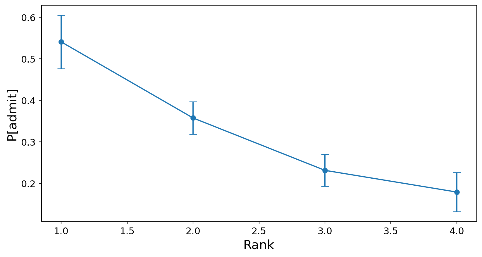
Note how
df.hist()automatically plots a histogram for each column in the dataframe as a subplot.
Let’s look at how each independent variable affects admission probability by plotting the mean admission probability as a function of the independent variable.
Note that there’s a greatly expanded
groupbysection in the Pandas refresher.
We add error bars to the means to indicate the standard error of the mean.
First, rank:
Code
import numpy as np

# Calculate mean and standard error
grouped = df.groupby('rank')['admit']
means = grouped.mean()

# Compute 'standard error of the mean'
errors = grouped.std() / np.sqrt(grouped.count())

# Plot with error bars
ax = means.plot(marker='o', yerr=errors, fontsize=12, capsize=5)
ax.set_ylabel('P[admit]', fontsize=16)
ax.set_xlabel('Rank', fontsize=16);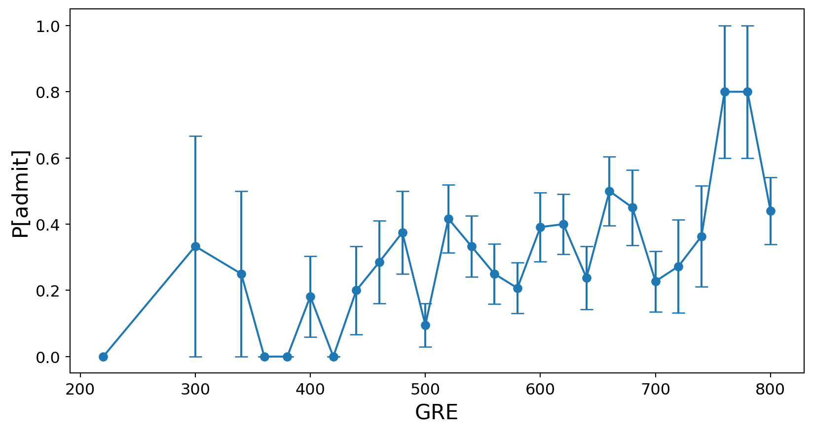
Next, GRE:
Code
grouped_gre = df.groupby('gre')['admit']
means_gre = grouped_gre.mean()
errors_gre = grouped_gre.std() / np.sqrt(grouped_gre.count())

ax = means_gre.plot(marker='o', yerr=errors_gre, fontsize=12, capsize=5)
ax.set_ylabel('P[admit]', fontsize=16)
ax.set_xlabel('GRE', fontsize=16);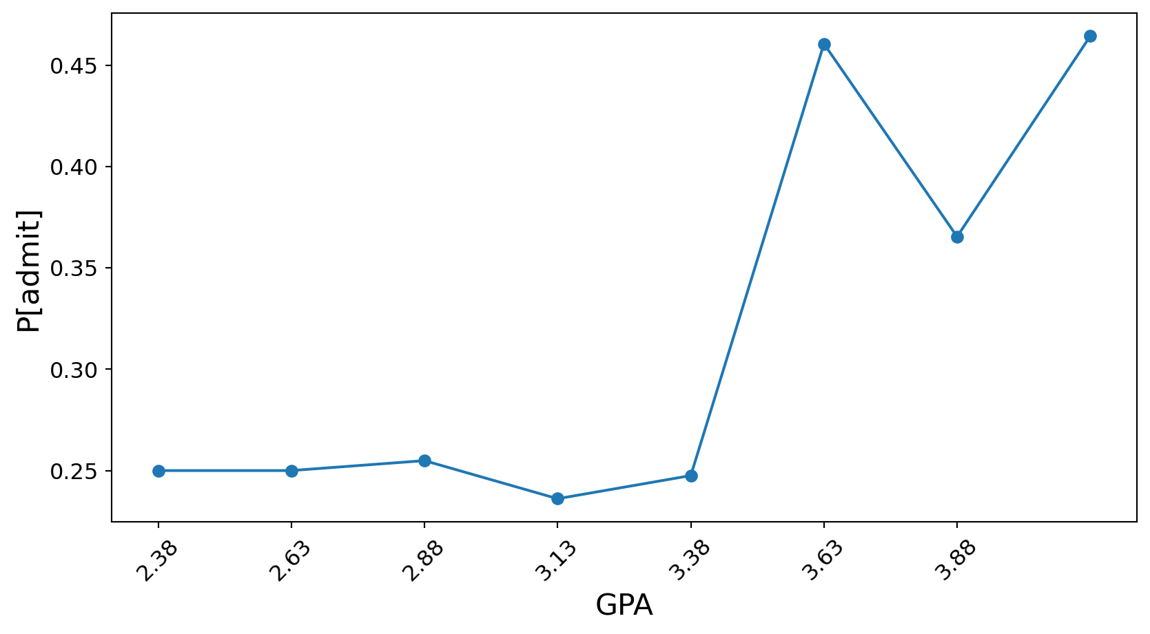
Finally, GPA (for this visualization, we aggregate GPA into 8 bins):
Code
bins = np.linspace(df.gpa.min(), df.gpa.max(), 8)
bin_centers = (bins[:-1] + bins[1:]) / 2
grouped_gpa = df.groupby(np.digitize(df.gpa, bins)).mean()['admit']
ax = grouped_gpa.plot(marker='o', fontsize=12)
ax.set_ylabel('P[admit]', fontsize=16)
ax.set_xlabel('GPA', fontsize=16)
ax.set_xticks(range(1, len(bin_centers) + 1))
ax.set_xticklabels([f'{center:.2f}' for center in bin_centers], rotation=45);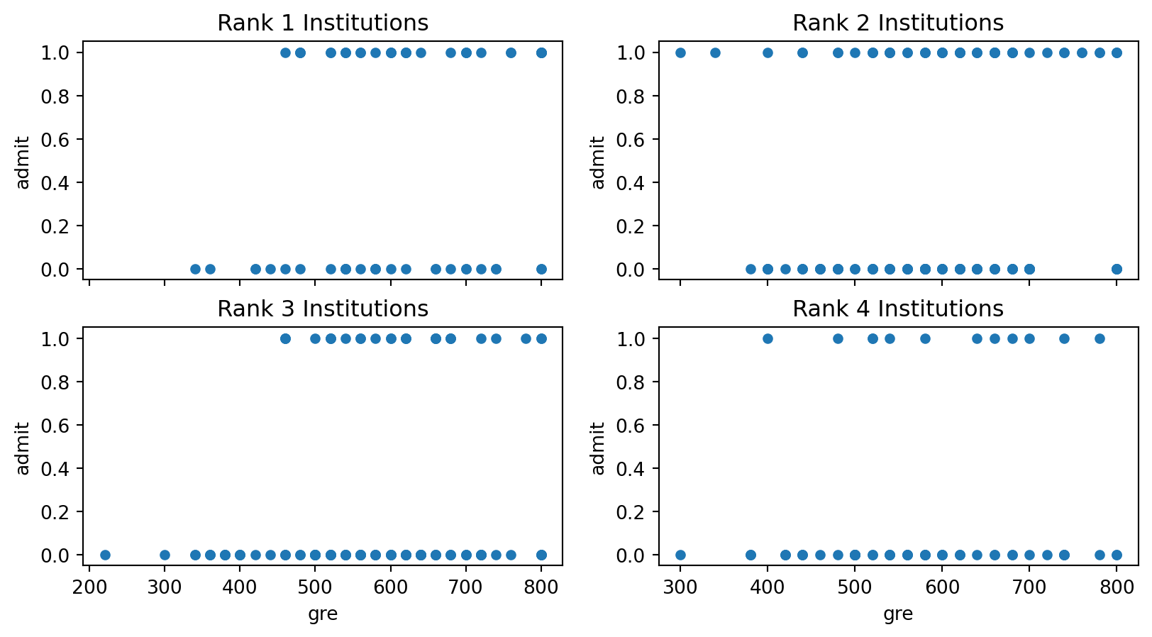
Finally, we plot admission status versus GRE score for each data point for each of the four ranks:
Code
df1 = df[df['rank']==1]
df2 = df[df['rank']==2]
df3 = df[df['rank']==3]
df4 = df[df['rank']==4]

fig = plt.figure(figsize = (10, 5))

ax1 = fig.add_subplot(221)
df1.plot.scatter('gre','admit', ax = ax1)
plt.title('Rank 1 Institutions')

ax2 = fig.add_subplot(222)
df2.plot.scatter('gre','admit', ax = ax2)
plt.title('Rank 2 Institutions')

ax3 = fig.add_subplot(223, sharex = ax1)
df3.plot.scatter('gre','admit', ax = ax3)
plt.title('Rank 3 Institutions')

ax4 = fig.add_subplot(224, sharex = ax2)
plt.title('Rank 4 Institutions')
df4.plot.scatter('gre','admit', ax = ax4);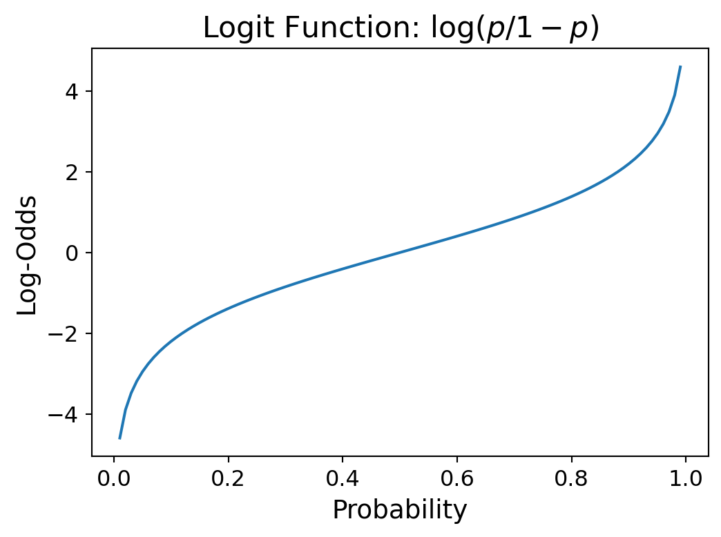
What we want to do is to fit a model that predicts the probability of admission as a function of these independent variables.
Logistic Regression
Logistic regression is concerned with estimating a probability.
However, all that is available are categorical observations, which we will code as 0/1.
That is, these could be pass/fail, admit/reject, Democrat/Republican, etc.
Now, a linear function like \(\beta_0 + \beta_1 x\) cannot be used to predict probability directly, because
- the linear function takes on all values (from -\(\infty\) to +\(\infty\)),
- and probability only ranges over \([0, 1]\).
Odds and Log-Odds
However, there is a transformation of probability that works: it is called log-odds.
For any probabilty \(p\), the odds is defined as \(p/(1-p)\), which is the ratio of the probability of an event to the probability of the non-event.
Notice that odds vary from 0 to \(\infty\), and odds < 1 indicates that \(p < 1/2\).
Now, there is a good argument that to fit a linear function, instead of using odds, we should use log-odds.
That is simply \(\log p/(1-p)\) which is also called the logit function, which is an abbreviation for logistic unit.
Code
pvec = np.linspace(0.01, 0.99, 100)
ax = plt.figure(figsize = (6, 4)).add_subplot()
ax.plot(pvec, np.log(pvec / (1-pvec)))
ax.tick_params(labelsize=12)
ax.set_xlabel('Probability', fontsize = 14)
ax.set_ylabel('Log-Odds', fontsize = 14)
ax.set_title('Logit Function: $\log (p/1-p)$', fontsize = 16);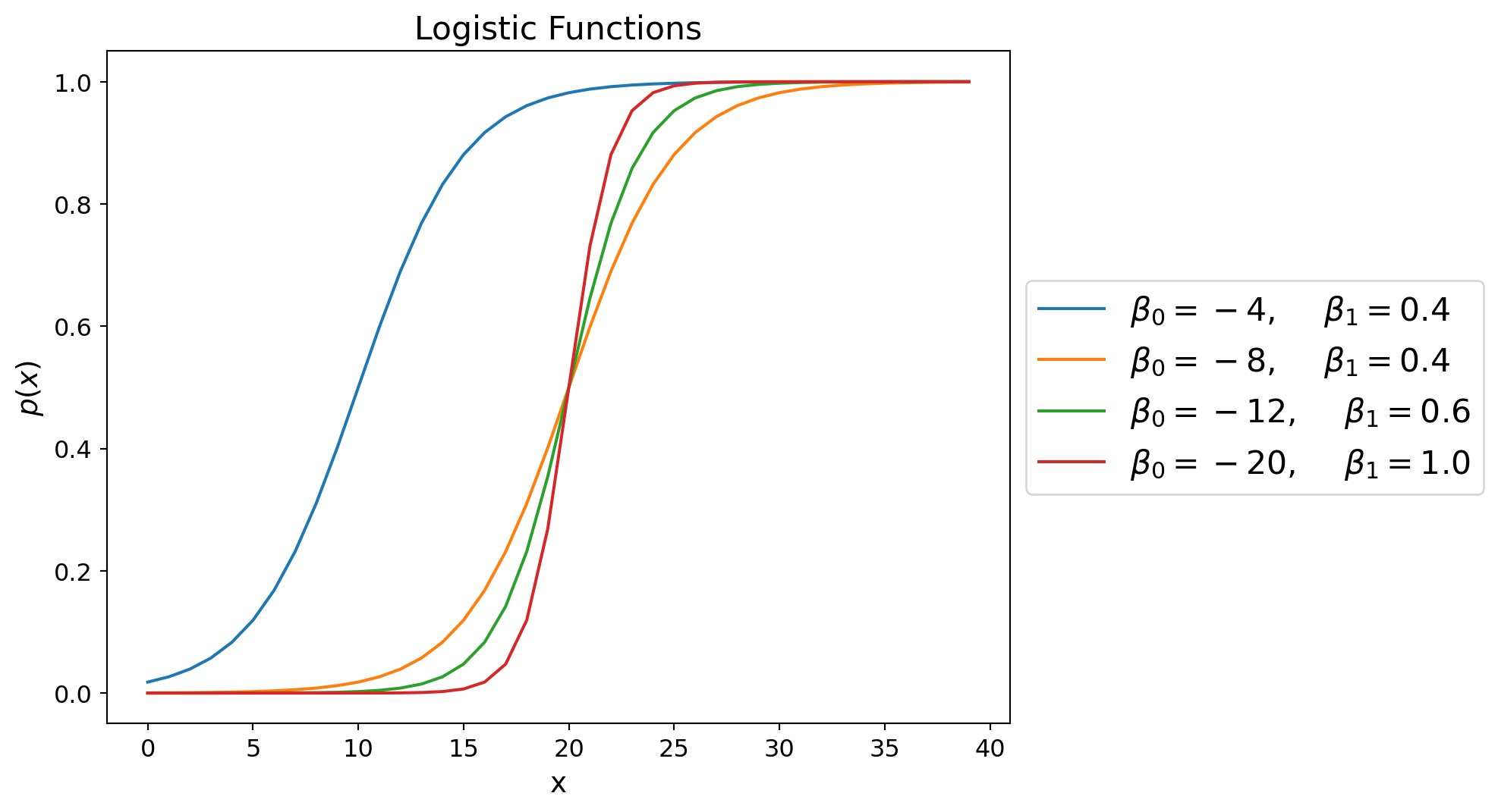
So, logistic regression does the following: it does a linear regression of \(\beta_0 + \beta_1 x\) against \(\log p/(1-p)\).
That is, it fits:
\[ \begin{aligned} \beta_0 + \beta_1 x &= \log \frac{p(x)}{1-p(x)} \\ e^{\beta_0 + \beta_1 x} &= \frac{p(x)}{1-p(x)} \quad \text{(exponentiate both sides)} \\ e^{\beta_0 + \beta_1 x} (1-p(x)) &= p(x) \quad \text{(multiply both sides by $1-p(x)$)} \\ e^{\beta_0 + \beta_1 x} &= p(x) + p(x)e^{\beta_0 + \beta_1 x} \quad \text{(distribute $p(x)$)} \\ \frac{e^{\beta_0 + \beta_1 x}}{1 +e^{\beta_0 + \beta_1 x}} &= p(x) \end{aligned} \]
So, logistic regression fits a probability of the following form:
\[ p(x) = P(y=1\mid x) = \frac{e^{\beta_0+\beta_1 x}}{1+e^{\beta_0+\beta_1 x}}. \]
This is a sigmoid function; when \(\beta_1 > 0\),
- as \(x\rightarrow \infty\), then \(p(x)\rightarrow 1\) and
- as \(x\rightarrow -\infty\), then \(p(x)\rightarrow 0\).
Holding \(\beta_0\) constant, we see that as \(\beta_1\) increases, the logistic function becomes steeper.
Code
alphas = [-4, -8,-12,-20]
alphas = [-8, -8, -8, -8]
betas = [0.2,0.4,0.6,1]
x = np.arange(40)
fig = plt.figure(figsize=(8, 6))
ax = plt.subplot(111)

for i in range(len(alphas)):
    a = alphas[i]
    b = betas[i]
    y = np.exp(a+b*x)/(1+np.exp(a+b*x))
#     plt.plot(x,y,label=r"$\frac{e^{%d + %3.1fx}}{1+e^{%d + %3.1fx}}\;\beta_0=%d, \beta_1=%3.1f$" % (a,b,a,b,a,b))
    ax.plot(x,y,label=r"$\beta_0=%d,$    $\beta_1=%3.1f$" % (a,b))
ax.tick_params(labelsize=12)
ax.set_xlabel('x', fontsize = 14)
ax.set_ylabel('$p(x)$', fontsize = 14)
ax.legend(loc='center left', bbox_to_anchor=(1, 0.5), prop={'size': 16})
ax.set_title('Logistic Functions', fontsize = 16);
Holding \(\beta_1\) constant, we see that as \(\beta_0\) increases, the logistic function shifts to the right.
Code
alphas = [-4, -8,-12,-20]
betas = [0.4, 0.4, 0.4, 0.4]
x = np.arange(40)
fig = plt.figure(figsize=(8, 6))
ax = plt.subplot(111)

for i in range(len(alphas)):
    a = alphas[i]
    b = betas[i]
    y = np.exp(a+b*x)/(1+np.exp(a+b*x))
#     plt.plot(x,y,label=r"$\frac{e^{%d + %3.1fx}}{1+e^{%d + %3.1fx}}\;\beta_0=%d, \beta_1=%3.1f$" % (a,b,a,b,a,b))
    ax.plot(x,y,label=r"$\beta_0=%d,$    $\beta_1=%3.1f$" % (a,b))
ax.tick_params(labelsize=12)
ax.set_xlabel('x', fontsize = 14)
ax.set_ylabel('$p(x)$', fontsize = 14)
ax.legend(loc='center left', bbox_to_anchor=(1, 0.5), prop={'size': 16})
ax.set_title('Logistic Functions', fontsize = 16);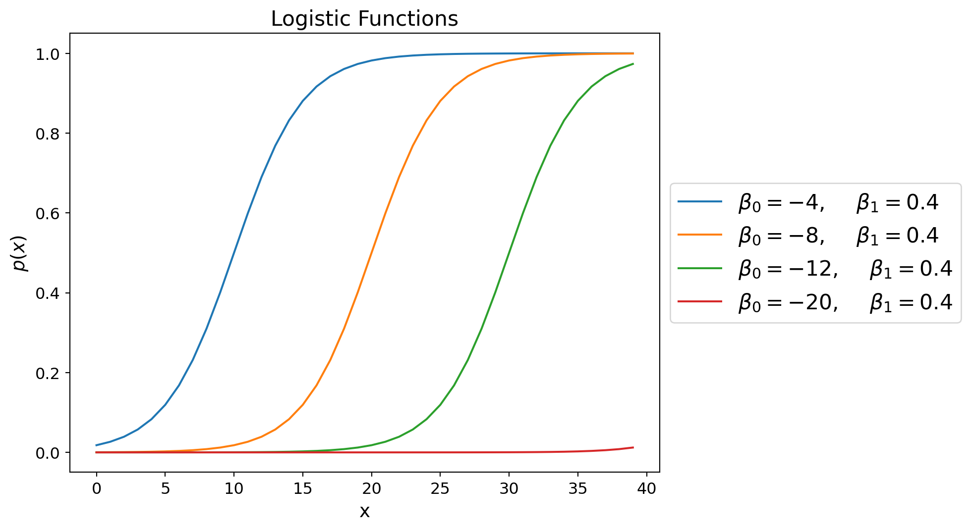
Varying both \(\beta_0\) and \(\beta_1\) gives us a more general logistic function.
Code
alphas = [-4, -8,-12,-20]
betas = [0.2,0.4,0.6,1]
x = np.arange(40)
fig = plt.figure(figsize=(8, 6))
ax = plt.subplot(111)

for i in range(len(alphas)):
    a = alphas[i]
    b = betas[i]
    y = np.exp(a+b*x)/(1+np.exp(a+b*x))
#     plt.plot(x,y,label=r"$\frac{e^{%d + %3.1fx}}{1+e^{%d + %3.1fx}}\;\beta_0=%d, \beta_1=%3.1f$" % (a,b,a,b,a,b))
    ax.plot(x,y,label=r"$\beta_0=%d,$    $\beta_1=%3.1f$" % (a,b))
ax.tick_params(labelsize=12)
ax.set_xlabel('x', fontsize = 14)
ax.set_ylabel('$p(x)$', fontsize = 14)
ax.legend(loc='center left', bbox_to_anchor=(1, 0.5), prop={'size': 16})
ax.set_title('Logistic Functions', fontsize = 16);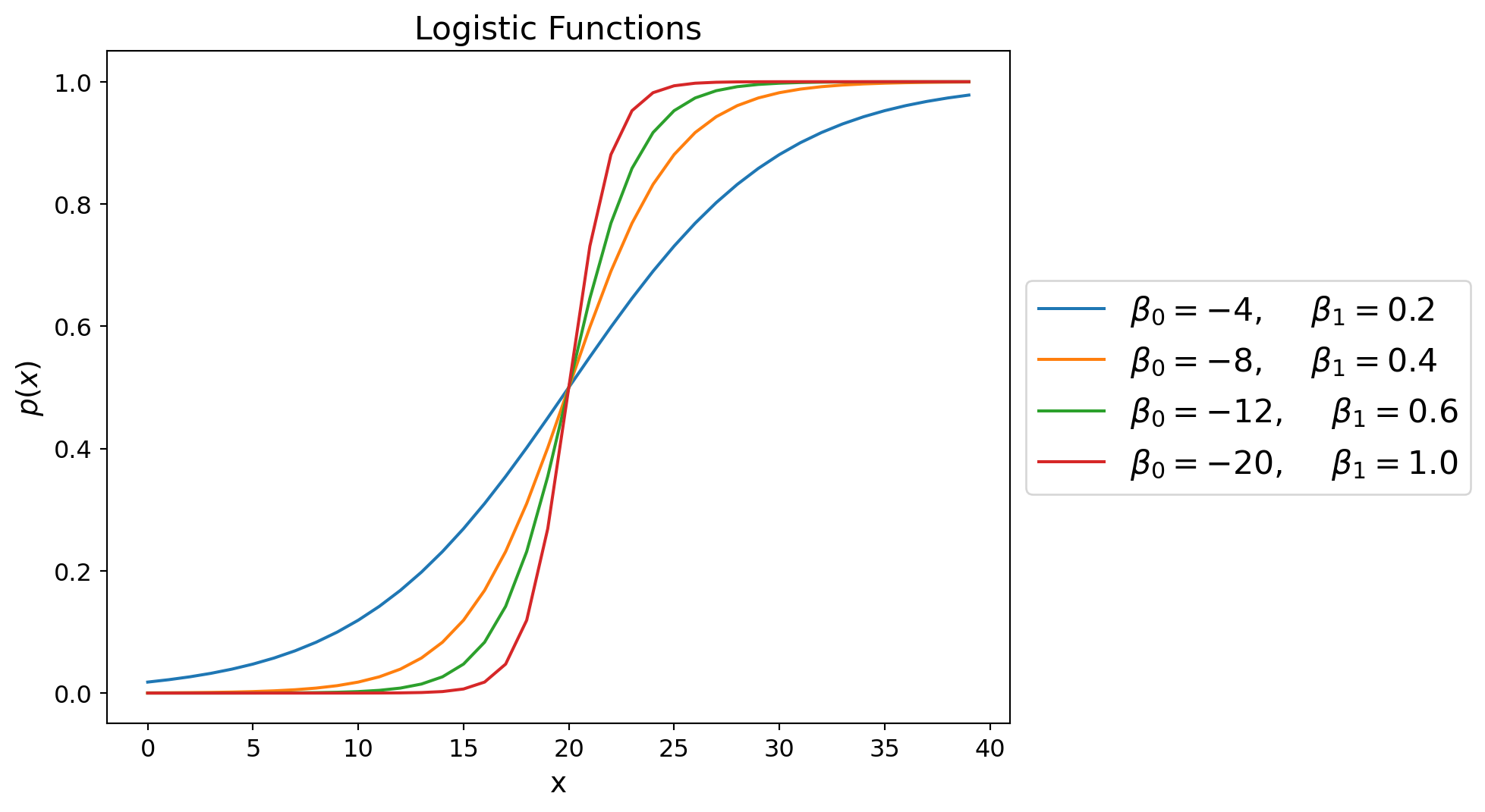
Parameter \(\beta_1\) controls how fast \(p(x)\) raises from \(0\) to \(1\)
The value of -\(\beta_0\)/\(\beta_1\) shows the value of \(x\) for which \(p(x)=0.5\)
Another interpretation of \(\beta_0\) is that it gives the base rate – the unconditional probability of a 1.
That is, if you knew nothing about a particular data item, then \(p(x) = 1/(1+e^{-\beta_0})\).
Code
# plot the base rate as a function of beta_0
beta_0_values = np.linspace(-10, 10, 100)
base_rate = 1 / (1 + np.exp(-beta_0_values))
plt.figure(figsize=(6, 4))
plt.plot(beta_0_values, base_rate)
plt.xlabel('beta_0')
plt.ylabel('Base Rate')
plt.title('Base Rate as a function of beta_0')
plt.show()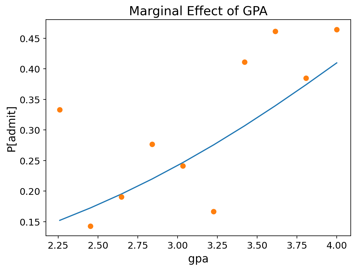
The function \(f(x) = \log (x/(1-x))\) is called the logit function.
So a compact way to describe logistic regression is that it finds regression coefficients \(\beta_0, \beta_1\) to fit:
\[ \text{logit}\left(p(x)\right)=\log\left(\frac{p(x)}{1-p(x)} \right) = \beta_0 + \beta_1 x. \]
Note also that the inverse logit function is:
\[ \text{logit}^{-1}(x) = \frac{e^x}{1 + e^x}. \]
Somewhat confusingly, this is called the logistic function.
So, the best way to think of logistic regression is that we compute a linear function:
\[ \beta_0 + \beta_1 x, \]
and then map that to a probability using the inverse \(\text{logit}\) function:
\[ \frac{e^{\beta_0+\beta_1 x}}{1+e^{\beta_0+\beta_1 x}}. \]
Logistic vs Linear Regression
Let’s take a moment to compare linear and logistic regression.
In Linear regression we fit
\[ y_i = \beta_0 +\beta_1 x_i + \epsilon_i. \]
We do the fitting by minimizing the sum of squared errors \(\Vert\epsilon\Vert\). This can be done in closed form using either geometric arguments or by calculus.
Now, if \(\epsilon_i\) comes from a normal distribution with mean zero and some fixed variance, then minimizing the sum of squared errors is exactly the same as finding the maximum likelihood of the data with respect to the probability of the errors.
So, in the case of linear regression, it is a lucky fact that the MLE of \(\beta_0\) and \(\beta_1\) can be found by a closed-form calculation.
In Logistic regression we fit
\[ \text{logit}(p(x_i)) = \beta_0 + \beta_1 x_i. \]
with \(\text{P}(y_i=1\mid x_i)=p(x_i).\)
How should we choose parameters?
Here too, we use Maximum Likelihood Estimation of the parameters.
That is, we choose the parameter values that maximize the likelihood of the data given the model.
\[ \text{P}(y_i \mid x_i) = \left\{\begin{array}{lr}\text{logit}^{-1}(\beta_0 + \beta_1 x_i)& \text{if } y_i = 1\\ 1 - \text{logit}^{-1}(\beta_0 + \beta_1 x_i)& \text{if } y_i = 0\end{array}\right. \]
We can write this as a single expression:
\[ \text{P}(y_i \mid x_i) = \text{logit}^{-1}(\beta_0 + \beta_1 x_i)^{y_i} (1-\text{logit}^{-1}(\beta_0 + \beta_1 x_i))^{1-y_i}, \]
where we assume the parameters are fixed.
We can reinterpret this to express the likelihood of parameters \(\beta_0\), \(\beta_1\):
\[ L(\beta_0, \beta_1 \mid x_i, y_i) = \text{logit}^{-1}(\beta_0 + \beta_1 x_i)^{y_i} (1-\text{logit}^{-1}(\beta_0 + \beta_1 x_i))^{1-y_i}, \]
given that we have observed the data \((x_i, y_i)\).
This is our objective function to maximize.
However, there is no closed-form solution so we optimize it numerically with gradient descent.
How Gradient Descent Works
Algorithm:
Initialize parameters: Start with random values \(\beta^{(0)}\)
Compute gradient: Calculate \(\nabla \ell(\beta^{(t)})\) - the direction of steepest increase
Update parameters: Take a step in that direction: \[\beta^{(t+1)} = \beta^{(t)} + \alpha \nabla \ell(\beta^{(t)})\] where \(\alpha\) is the learning rate (step size)
Repeat steps 2-3 until convergence (gradient \(\approx 0\) or max iterations reached)
Result: Parameters that (locally) maximize the likelihood of the observed data.
Logistic Regression In Practice
So, in summary, we have:
Input pairs \((x_i,y_i)\)
Output parameters \(\widehat{\beta_0}\) and \(\widehat{\beta_1}\) that maximize the likelihood of the data given these parameters for the logistic regression model.
Method Maximum likelihood estimation, obtained by gradient descent.
The standard package will give us a coefficient \(\beta_i\) for each independent variable (feature).
If we want to include a constant (i.e., \(\beta_0\)) we need to add a column of 1s (just like in linear regression).
Code
df['intercept'] = 1.0
train_cols = df.columns[1:]
train_cols
Index(['gre', 'gpa', 'rank', 'intercept'], dtype='object')Code
logit = sm.Logit(df['admit'], df[train_cols])

# fit the model
result = logit.fit()
Optimization terminated successfully.
Current function value: 0.574302
Iterations 6Statsmodels gives us a summary of the model fit.
Code
result.summary()| Dep. Variable: | admit | No. Observations: | 400 |
|---|---|---|---|
| Model: | Logit | Df Residuals: | 396 |
| Method: | MLE | Df Model: | 3 |
| Date: | Tue, 28 Oct 2025 | Pseudo R-squ.: | 0.08107 |
| Time: | 10:40:08 | Log-Likelihood: | -229.72 |
| converged: | True | LL-Null: | -249.99 |
| Covariance Type: | nonrobust | LLR p-value: | 8.207e-09 |
| coef | std err | z | P>|z| | [0.025 | 0.975] | |
|---|---|---|---|---|---|---|
| gre | 0.0023 | 0.001 | 2.101 | 0.036 | 0.000 | 0.004 |
| gpa | 0.7770 | 0.327 | 2.373 | 0.018 | 0.135 | 1.419 |
| rank | -0.5600 | 0.127 | -4.405 | 0.000 | -0.809 | -0.311 |
| intercept | -3.4495 | 1.133 | -3.045 | 0.002 | -5.670 | -1.229 |
Notice that all of our independent variables are considered significant (no confidence intervals contain zero).
Using the Model
Note that by fitting a model to the data, we can make predictions for inputs that were not in the training data.
Furthermore, we can make a prediction of a probability for cases where we don’t have enough data to estimate the probability directly – e.g., for specific parameter values.
Let’s see how well the model fits the data.
We have three independent variables, so in each case we’ll use average values for the two that we aren’t evaluating.
GPA (GRE = 600, Rank = 2.5):
Code
bins = np.linspace(df.gpa.min(), df.gpa.max(), 10)
groups = df.groupby(np.digitize(df.gpa, bins))
prob = [result.predict([600, b, 2.5, 1.0]) for b in bins]
ax = plt.figure(figsize = (7, 4)).add_subplot()
ax.plot(bins, prob)
ax.plot(bins,groups.admit.mean(),'o')
ax.tick_params(labelsize=12)
ax.set_xlabel('gpa', fontsize = 14)
ax.set_ylabel('P[admit]', fontsize = 14)
ax.set_title('Marginal Effect of GPA', fontsize = 16);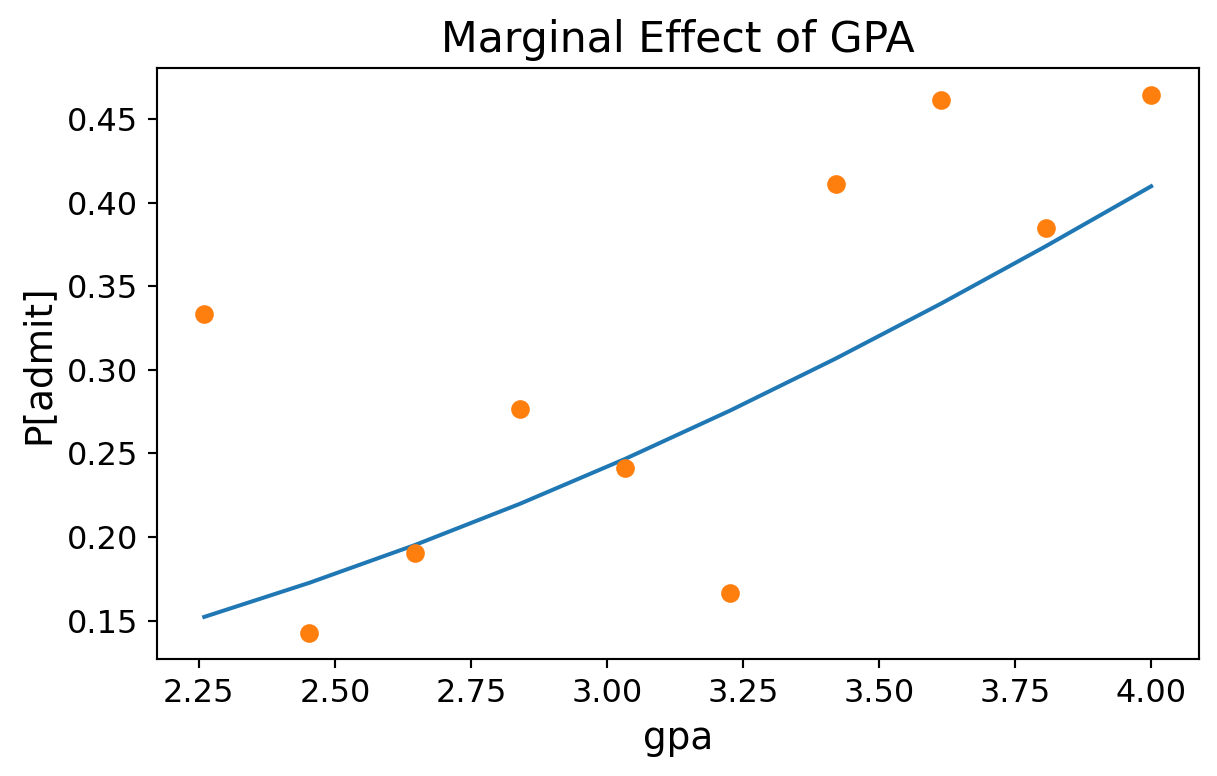
GRE Score (GPA = 3.4, Rank = 2.5):
Code
prob = [result.predict([b, 3.4, 2.5, 1.0]) for b in sorted(df.gre.unique())]
ax = plt.figure(figsize = (7, 4)).add_subplot()
ax.plot(sorted(df.gre.unique()), prob)
ax.plot(df.groupby('gre').mean()['admit'],'o')
ax.tick_params(labelsize=12)
ax.set_xlabel('gre', fontsize = 14)
ax.set_ylabel('P[admit]', fontsize = 14)
ax.set_title('Marginal Effect of GRE', fontsize = 16);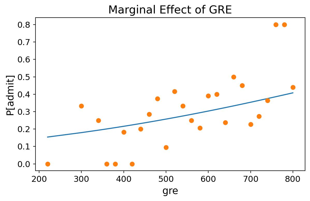
Institution Rank (GRE = 600, GPA = 3.4):
Code
prob = [result.predict([600, 3.4, b, 1.0]) for b in range(1,5)]
ax = plt.figure(figsize = (7, 4)).add_subplot()
ax.plot(range(1,5), prob)
ax.plot(df.groupby('rank').mean()['admit'],'o')
ax.tick_params(labelsize=12)
ax.set_xlabel('Rank', fontsize = 14)
ax.set_xlim([0.5,4.5])
ax.set_ylabel('P[admit]', fontsize = 14)
ax.set_title('Marginal Effect of Rank', fontsize = 16);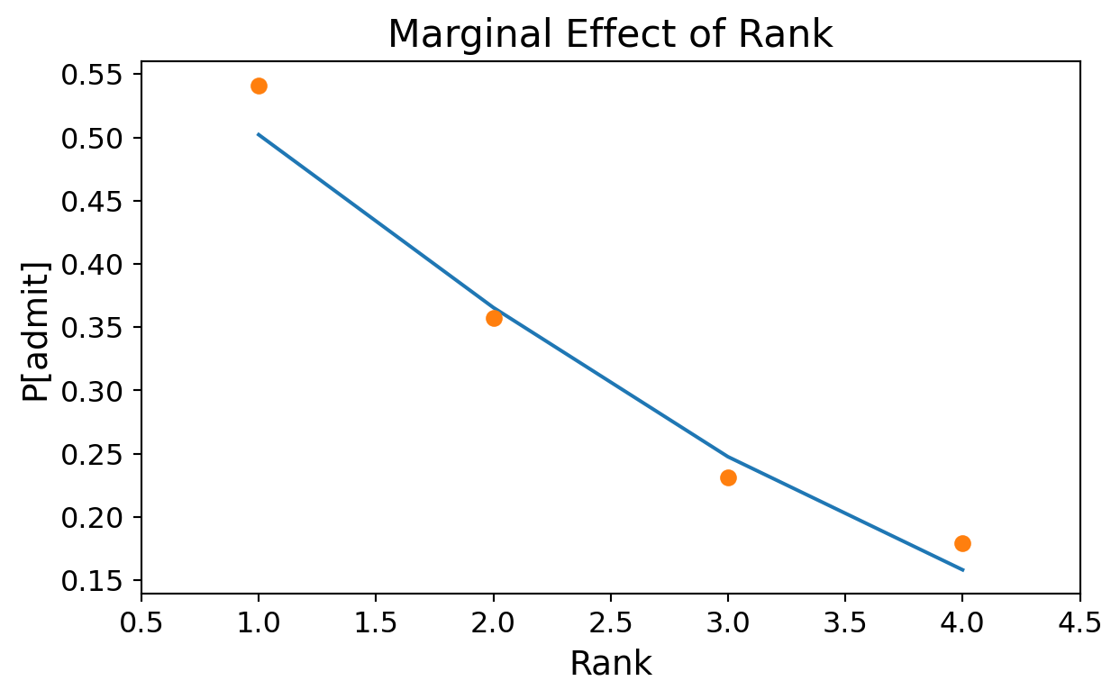
Logistic Regression in Perspective
At the start of lecture we emphasized that logistic regression is concerned with estimating a probability model for discrete (0/1) data.
However, it may well be the case that we want to do something with the probability that amounts to classification.
For example, we may classify data items using a rule such as “Assign item \(x_i\) to Class 1 if \(p(x_i) > 0.5\)”.
For this reason, logistic regression could be considered a classification method.
Let’s use our logistic regression as a classifier.
We want to ask whether we can correctly predict whether a student gets admitted to graduate school.
Let’s separate our training and test data:
Code
X_train, X_test, y_train, y_test = model_selection.train_test_split(
        df[train_cols], df['admit'],
        test_size=0.4, random_state=1)
Now, there are some standard metrics used when evaluating a binary classifier.
Let’s say our classifier is outputting “yes” when it thinks the student will be admitted.
There are four cases:
- Classifier says “yes”, and student is admitted: True Positive.
- Classifier says “yes”, and student is not admitted: False Positive.
- Classifier says “no”, and student is admitted: False Negative.
- Classifier says “no”, and student is not admitted: True Negative.
Precision is the fraction of “yes” classifications that are correct:
\[ \mbox{Precision} = \frac{\mbox{True Positives}}{\mbox{True Positives + False Positives}}. \]
Recall is the fraction of admits that we say “yes” to:
\[ \mbox{Recall} = \frac{\mbox{True Positives}}{\mbox{True Positives + False Negatives}}. \]
Code
def evaluate(y_train, X_train, y_test, X_test, threshold):

    # learn model on training data
    logit = sm.Logit(y_train, X_train)
    result = logit.fit(disp=False)

    # make probability predictions on test data
    y_pred = result.predict(X_test)

    # threshold probabilities to create classifications
    y_pred = y_pred > threshold

    # report metrics
    precision = metrics.precision_score(y_test, y_pred)
    recall = metrics.recall_score(y_test, y_pred)
    return precision, recall

precision, recall = evaluate(y_train, X_train, y_test, X_test, 0.5)

print(f'Precision: {precision:0.3f}, Recall: {recall:0.3f}')
Precision: 0.586, Recall: 0.340Now, let’s get a sense of average accuracy:
Code
PR = []
for i in range(20):
    X_train, X_test, y_train, y_test = model_selection.train_test_split(
            df[train_cols], df['admit'],
            test_size=0.4)
    PR.append(evaluate(y_train, X_train, y_test, X_test, 0.5))
Code
avgPrec = np.mean([f[0] for f in PR])
avgRec = np.mean([f[1] for f in PR])
print(f'Average Precision: {avgPrec:0.3f}, Average Recall: {avgRec:0.3f}')
Average Precision: 0.571, Average Recall: 0.211Sometimes we would like a single value that describes the overall performance of the classifier.
For this, we take the harmonic mean of precision and recall, called F1 Score:
\[ \mbox{F1 Score} = 2 \;\;\frac{\mbox{Precision} \cdot \mbox{Recall}}{\mbox{Precision} + \mbox{Recall}}. \]
Using this, we can evaluate other settings for the threshold.
Code
import warnings
warnings.filterwarnings("ignore")
def evalThresh(df, thresh):
    PR = []
    for i in range(20):
        X_train, X_test, y_train, y_test = model_selection.train_test_split(
                df[train_cols], df['admit'],
                test_size=0.4)
        PR.append(evaluate(y_train, X_train, y_test, X_test, thresh))
    avgPrec = np.mean([f[0] for f in PR])
    avgRec = np.mean([f[1] for f in PR])
    return 2 * (avgPrec * avgRec) / (avgPrec + avgRec), avgPrec, avgRec

tvals = np.linspace(0.05, 0.8, 50)
f1vals = [evalThresh(df, tval)[0] for tval in tvals]
Code
plt.figure(figsize=(6, 3))
plt.plot(tvals,f1vals)
plt.ylabel('F1 Score')
plt.xlabel('Threshold for Classification')
plt.title('F1 as a function of Threshold');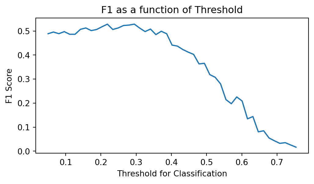
Based on this plot, we can say that the best classification threshold appears to be around 0.3, where precision and recall are:
Code
F1, Prec, Rec = evalThresh(df, 0.3)
print('Best Precision: {:0.3f}, Best Recall: {:0.3f}'.format(Prec, Rec))
Best Precision: 0.426, Best Recall: 0.677The example here is based on http://blog.yhathq.com/posts/logistic-regression-and-python.html where you can find additional details.
ROC-AUC Curve
The ROC-AUC curve is a plot of the true positive rate against the false positive rate at various threshold settings.
The AUC is the area under the ROC curve.
The AUC is a measure of the overall performance of the classifier.
Code
# Get predicted probabilities from the model
y_pred_proba = result.predict(df[train_cols])

# Compute ROC curve and AUC
fpr, tpr, thresholds = metrics.roc_curve(df['admit'], y_pred_proba)
auc_score = metrics.roc_auc_score(df['admit'], y_pred_proba)

# Plot ROC curve
fig, ax = plt.subplots(figsize=(4, 4))
ax.plot(fpr, tpr, linewidth=2, label=f'ROC curve (AUC = {auc_score:.3f})')
ax.plot([0, 1], [0, 1], 'k--', linewidth=1, label='Random classifier')
ax.set_xlabel('False Positive Rate', fontsize=12)
ax.set_ylabel('True Positive Rate', fontsize=12)
ax.set_title('ROC Curve for Logistic Regression Model', fontsize=14)
ax.legend(loc='lower right', fontsize=11)
ax.grid(True, alpha=0.3)
ax.tick_params(labelsize=11)
plt.tight_layout()
plt.show()

print(f"AUC Score: {auc_score:.4f}")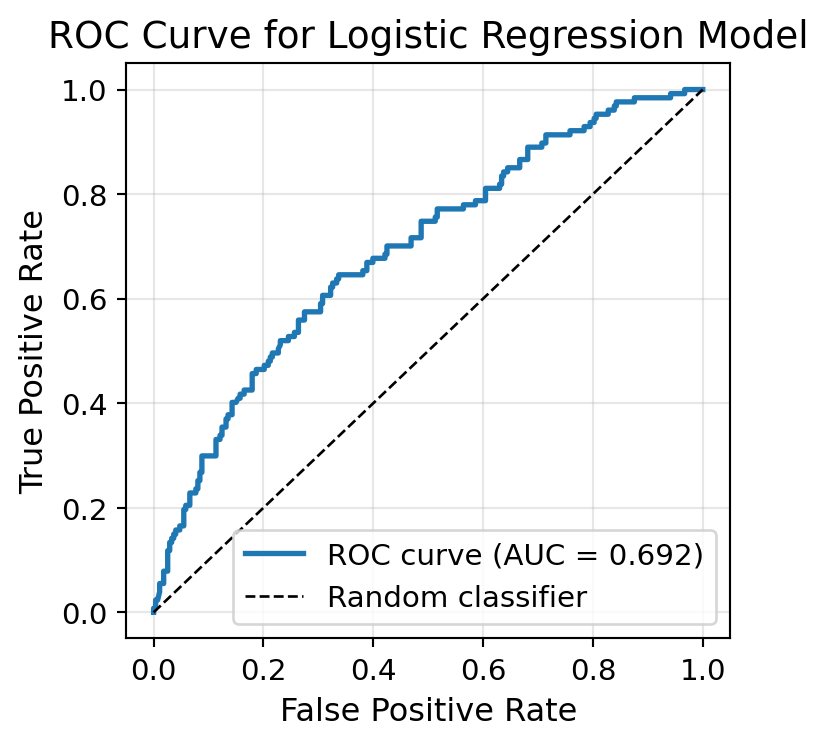
AUC Score: 0.6921Recap
- Logistic regression is used to predict a probability.
- It is a linear model for the log-odds.
- It is fit by maximum likelihood.
- It can be evaluated as a classifier.