| Home Owner | Marital Status | Annual Income | Defaulted Borrower | |
|---|---|---|---|---|
| ID | ||||
| 1 | Yes | Single | 125000 | No |
| 2 | No | Married | 100000 | No |
| 3 | No | Single | 70000 | No |
| 4 | Yes | Married | 120000 | No |
| 5 | No | Divorced | 95000 | Yes |
| 6 | No | Married | 60000 | No |
| 7 | Yes | Divorced | 220000 | No |
| 8 | No | Single | 85000 | Yes |
| 9 | No | Married | 75000 | No |
| 10 | No | Single | 90000 | Yes |
Decision Trees and Random Forests
Outline
![]()
- Build a decision tree manually
- Look at single and collective impurity measures
- Selecting splitting attributes and test conditions
- Scikit-learn implementation
- Model training and evaluation
- Bias and Variance
- Random forests
Introduction
We’ll now start looking into how to build models to predict an outcome variable from labeled data.
Classification problems:
- predict a category
- e.g., spam/not spam, fraud/not fraud, default/not default, malignant/benign, etc.
Regression problems:
- predict a numeric value
- e.g., price of a house, salary of a person, etc.
Loan Default Example
We’ll use an example from (Tan et al. 2018).
![]()
You are a loan officer at Terrier Savings and Loan.
You have a dataset on loans that you have made in the past.
You want to build a model to predict whether a loan will default.
Loans Data Set
Loans Data Set Summary
Here’s the summary info of the data set.
Code
loans.info()<class 'pandas.core.frame.DataFrame'>
Index: 10 entries, 1 to 10
Data columns (total 4 columns):
# Column Non-Null Count Dtype
--- ------ -------------- -----
0 Home Owner 10 non-null object
1 Marital Status 10 non-null object
2 Annual Income 10 non-null int64
3 Defaulted Borrower 10 non-null object
dtypes: int64(1), object(3)
memory usage: 400.0+ bytesConvert to Categorical Data Types
Since some of the fields are categorical, let’s convert them to categorical data types.
loans['Home Owner'] = loans['Home Owner'].astype('category')
loans['Marital Status'] = loans['Marital Status'].astype('category')
loans['Defaulted Borrower'] = loans['Defaulted Borrower'].astype('category')
loans.info()
<class 'pandas.core.frame.DataFrame'>
Index: 10 entries, 1 to 10
Data columns (total 4 columns):
# Column Non-Null Count Dtype
--- ------ -------------- -----
0 Home Owner 10 non-null category
1 Marital Status 10 non-null category
2 Annual Income 10 non-null int64
3 Defaulted Borrower 10 non-null category
dtypes: category(3), int64(1)
memory usage: 570.0 bytesSimple Model
Looking at the table, let’s just start with the simplest model possible and just predict that no one will default.
So the output of our model is just to always predict “No”.

We see a 30% error rate since 3 out of 10 loans defaulted.
Let’s split the data based on the “Home Owner” field. (values = [# No, # Yes]).

We see that the left node (Home Owner == Yes) has a 0% error rate since all the samples are Defaulted == No. We don’t split this node since all the samples are of the same class. We call this node a leaf node and we’ll color it orange.
The right node (Home Owner == No) has a 43% error rate since 3 out of 7 loans defaulted.
Let’s split this node into two nodes based on the Marital Status field.
Let’s split on the “Marital Status” field.
We see that the 3 defaulted loans are all for single or divorced people. Since the node is all one class, we don’t split this node and we call it a leaf node.

We can list the subsets for the two criteria to calculate the error rate.
Code
loans[(loans['Home Owner'] == "No") & (loans['Marital Status'].isin(['Single', 'Divorced']))]| Home Owner | Marital Status | Annual Income | Defaulted Borrower | |
|---|---|---|---|---|
| ID | ||||
| 3 | No | Single | 70000 | No |
| 5 | No | Divorced | 95000 | Yes |
| 8 | No | Single | 85000 | Yes |
| 10 | No | Single | 90000 | Yes |
Table: Home Owner == No and Marital Status == Single or Divorced –> Defaulted == Yes
Error rate for predicting Defaulted == Yes is 25%.
and…
Code
loans[(loans['Home Owner'] == "No") & (loans['Marital Status'] == "Married")]| Home Owner | Marital Status | Annual Income | Defaulted Borrower | |
|---|---|---|---|---|
| ID | ||||
| 2 | No | Married | 100000 | No |
| 6 | No | Married | 60000 | No |
| 9 | No | Married | 75000 | No |
Table: Home Owner == No and Marital Status == Married –> Defaulted == No
Error rate for predicting Defaulted == No is 0%.
Let’s try to split on the “Annual Income” field.
We see that the person with income of 70K doesn’t default, so we split the node into two nodes based on the “Income” field.
We arbitrarily pick a threshold of $75K.

Evaluating the Model
We’ve dispositioned every data point by walking down the tree to a leaf node.
How do we know if this tree is good?
- We arbitrarily picked the order of the fields to split on.
Is there a way to systematically pick the order of the fields to split on?
- This is called the splitting criterion.
There’s also the question of when to stop splitting, or the stopping criterion.
So far, we stopped splitting when we reached a node of pure class but there are reasons to stop splitting even without pure classes, which we’ll see later.
Specifying the Test Condition
Before we continue, we should take a moment to consider how we specify a test condition of a node.
How we specify a test condition depends on the attribute type which can be:
- Binary (Boolean)
- Nominal (Categorical, e.g., cat, dog, bird)
- Ordinal (e.g., Small, Medium, Large)
- Continuous (e.g., 1.5, 2.1, 3.7)
And depends on the number of ways to split:
- multi-way
- binary
For a Nominal (Categorical) attribute:
- In a Multi-way split we can use as many partitions as there are distinct values of the attribute:

For a Nominal (Categorical) attribute:
In a Binary split we divide the values into two groups.
In this case, we need to find an optimal partitioning of values into groups, which we discuss shortly.


For an Ordinal attribute, we can use a multi-way split with as many partitions as there are distinct values.

Or we can use a binary split as long we preserve the ordering of the values.


Warning
Be careful not to violate the ordering of values such as {Small, Large} and {Medium, X-Large}.
A Continuous attribute can be handled two ways:


Note that finding good partitions for \(k\) nominal attributes can be expensive, \(\mathcal{O}(2^k)\), possibly involving combinatorial searching of groupings.
However for ordinal or continuous attributes, sweeping through a range of \(n\) threshold values can be more efficient if \(n \approx k\). \(\mathcal{O}(n)\) for a sorted list.
Selecting Attribute and Test Condition
Ideally, we want to pick attributes and test conditions that maximize the homogeneity of the splits.
We can use an impurity index to measure the homogeneity in a node.
We’ll look at ways of measuring impurity of a node and then collective impurity of its child nodes.
Impurity Measures
The following are three impurity indices:
\[ \begin{aligned} \textnormal{Gini index} &= 1 - \sum_{i=0}^{c-1} p_i(t)^2 \\ \textnormal{Entropy} &= -\sum_{i=0}^{c-1} p_i(t) \log_2 p_i(t) \\ \textnormal{Classification error} &= 1 - \max_i p_i(t) \end{aligned} \]
where \(p_i(t)\) is the relative frequency of training instances of class \(i\) at a node \(t\) and \(c\) is the number of classes.
Note
By convention, we set \(0 \log_2 0 = 0\) in entropy calculations.
Impurity Measures
The following are three impurity indices:
\[ \begin{aligned} \textnormal{Gini index} &= 1 - \sum_{i=0}^{c-1} p_i(t)^2 \\ \textnormal{Entropy} &= -\sum_{i=0}^{c-1} p_i(t) \log_2 p_i(t) \\ \textnormal{Classification error} &= 1 - \max_i p_i(t) \end{aligned} \]
All three impurity indices equal 0 when all the records at a node belong to the same class.
All three impurity indices reach their maximum value when the classes are evenly distributed among the child nodes.
We can plot the three impurity indices to get a sense of how they behave for binary classification problems.
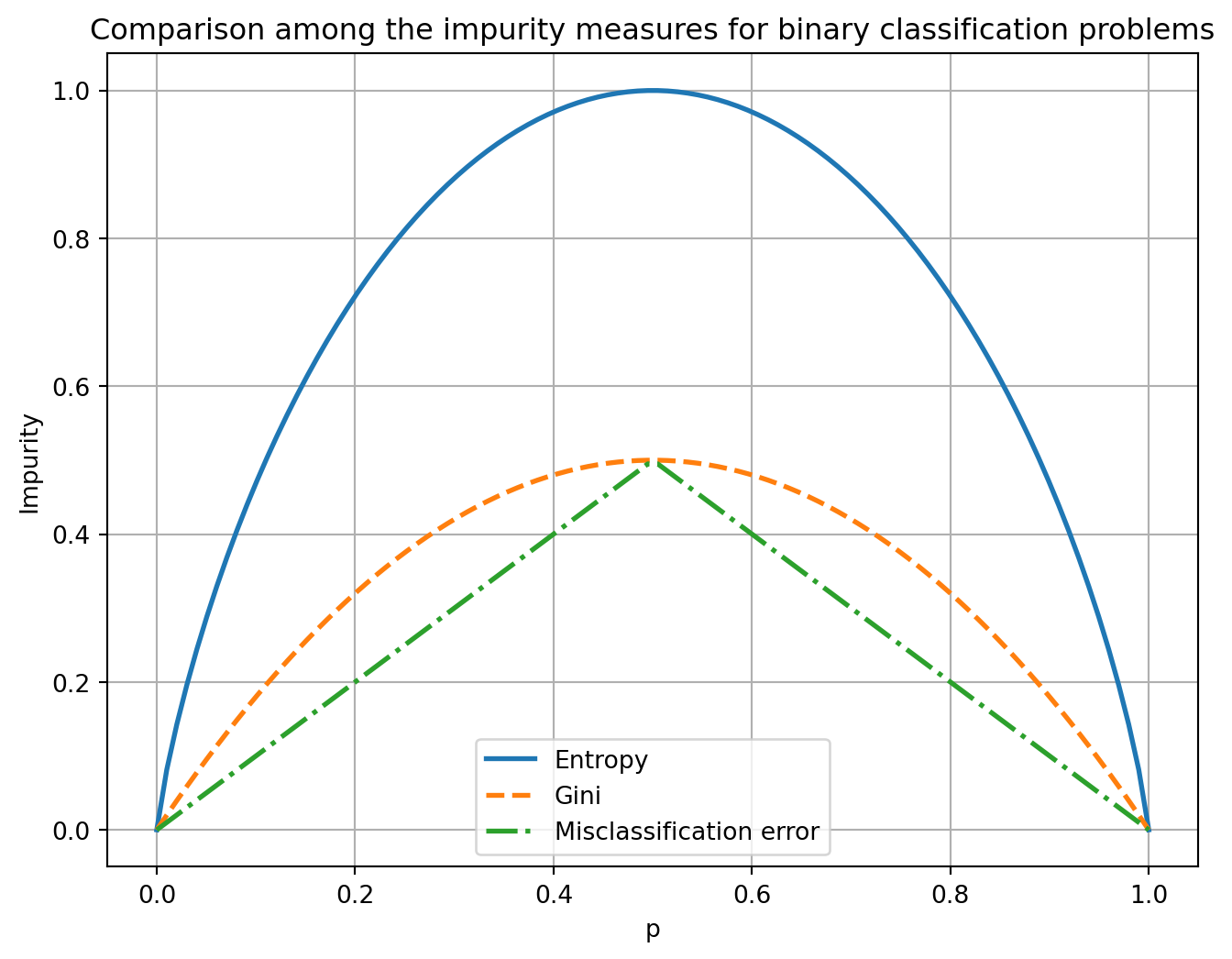
They all maintain the same ordering for every relative frequency, i.e., Entropy > Gini > Misclassification error.
Impurity Example 1
| Node \(N_1\) | Count | p |
|---|---|---|
| Class=0 | 0 | \(0/6 = 0\) |
| Class=1 | 6 | \(6/6 = 1\) |
\[ \begin{aligned} \textnormal{Gini} &= 1 - \left(\frac{0}{6}\right)^2 - \left(\frac{6}{6}\right)^2 = 0 \\ \textnormal{Entropy} &= -\left(\frac{0}{6} \log_2 \frac{0}{6} + \frac{6}{6} \log_2 \frac{6}{6}\right) = 0 \\ \textnormal{Error} &= 1 - \max\left[\frac{0}{6}, \frac{6}{6}\right] = 0 \end{aligned} \]
Impurity Example 2
| Node \(N_2\) | Count | p |
|---|---|---|
| Class=0 | 1 | \(1/6 = 0.167\) |
| Class=1 | 5 | \(5/6 = 0.833\) |
\[ \begin{aligned} \textnormal{Gini} &= 1 - \left(\frac{1}{6}\right)^2 - \left(\frac{5}{6}\right)^2 = 0.278 \\ \textnormal{Entropy} &= -\left(\frac{1}{6} \log_2 \frac{1}{6} + \frac{5}{6} \log_2 \frac{5}{6}\right) = 0.650 \\ \textnormal{Error} &= 1 - \max\left[\frac{1}{6}, \frac{5}{6}\right] = 0.167 \end{aligned} \]
Impurity Example 3
| Node \(N_3\) | Count |
|---|---|
| Class=0 | 3 |
| Class=1 | 3 |
\[ \begin{aligned} \textnormal{Gini} &= 1 - \left(\frac{3}{6}\right)^2 - \left(\frac{3}{6}\right)^2 = 0.5 \\ \textnormal{Entropy} &= -\left(\frac{3}{6} \log_2 \frac{3}{6} + \frac{3}{6} \log_2 \frac{3}{6}\right) = 1 \\ \textnormal{Error} &= 1 - \max\left[\frac{3}{6}, \frac{3}{6}\right] = 0.5 \end{aligned} \]
Impurity Class Exercise
Calculate Gini impurity for the following node:
| Node \(N_4\) | Count | p |
|---|---|---|
| Class=0 | 3 | |
| Class=1 | 6 | |
| Class=2 | 1 |
\[ \textnormal{Gini} = \]
Collective Impurity of Child Nodes
We can compute the collective impurity of child nodes by taking a weighted sum of the impurities of the child nodes.
\[ I(\textnormal{children}) = \sum_{j=1}^{k} \frac{N(v_j)}{N}\; I(v_j) \]
Here we split \(N\) training instances into \(k\) child nodes, \(v_j\) for \(j=1, \ldots, k\).
\(N(v_j)\) is the number of training instances at child node \(v_j\) and \(I(v_j)\) is the impurity at child node \(v_j\).
Impurity Example
Let’s compute collective impurity on our loans dataset to see which feature to split on.


Tip
Try calculating the collective Entropy for (a) and (b) and see if you get the same values.
Important
The collective entropy for (c) is 0. Why would we not want to use this node?
There are two ways to overcome this problem.
- One way is to generate only binary decision trees, thus avoiding the difficulty of handling attributes with varying number of partitions. This strategy is employed by decision tree classifiers such as CART.
- Another way is to modify the splitting criterion to take into account the number of partitions produced by the attribute. For example, in the C4.5 decision tree algorithm, a measure known as gain ratio is used to compensate for attributes that produce a large number of child nodes.
CART stands for Classification And Regression Tree.
Gain Ratio
See (Tan et al. 2018, chap. 3, p. 127):
- Having a low impurity value alone is insufficient to find a good attribute test condition for a node.
- Having more child nodes can make a decision tree more complex and consequently more susceptible to overfitting.
Hence, the number of children produced by the splitting attribute should also be taken into consideration while deciding the best attribute test condition.
Gain Ratio Formula
\[ \text{Gain ratio} = \frac{\Delta_{\text{info}}}{\text{Split Info}} = \frac{\text{Entropy(Parent)} - \sum_{i=1}^{k} \frac{N(v_i)}{N} \text{Entropy}(v_i)}{- \sum_{i=1}^{k} \frac{N(v_i)}{N} \log_2 \frac{N(v_i)}{N}} \]
where \(N(v_i)\) is the number of instances assigned to node \(v_i\) and \(k\) is the total number of splits.
The split information measures the entropy of splitting a node into its child nodes and evaluates if the split results in a larger number of equally-sized child nodes or not.
Gain Ratio Example
Let’s compare the Gain Ratio for Home Owner and Marital Status attributes using the loans dataset.
Recall from the earlier example that the parent node has 3 Yes and 7 No defaulters (10 total instances).
Parent node entropy:
\[ \text{Entropy(Parent)} = -\frac{3}{10} \log_2 \frac{3}{10} - \frac{7}{10} \log_2 \frac{7}{10} = 0.881 \]
Ex: Gain Ratio for Home Owner Attribute
The Home Owner attribute splits the data into 2 child nodes:
- Yes: 0 Yes, 3 No (3 instances)
- No: 3 Yes, 4 No (7 instances)
From the earlier calculation, the Information Gain is:
\[ \Delta_{\text{info}} = 0.881 - \left(\frac{3}{10} \times 0 + \frac{7}{10} \times 0.985\right) = 0.192 \]
Now we calculate the Split Information:
\[ \text{Split Info} = -\frac{3}{10} \log_2 \frac{3}{10} - \frac{7}{10} \log_2 \frac{7}{10} = 0.881 \]
Therefore, the Gain Ratio is:
\[ \text{Gain Ratio(Home Owner)} = \frac{0.192}{0.881} = 0.218 \]
Ex: Gain Ratio for Marital Status Attribute
The Marital Status attribute splits the data into 3 child nodes:
- Single: 2 Yes, 3 No (5 instances)
- Married: 0 Yes, 3 No (3 instances)
- Divorced: 1 Yes, 1 No (2 instances)
From the earlier calculation, the Information Gain is:
\[ \Delta_{\text{info}} = 0.881 - \left(\frac{5}{10} \times 0.971 + \frac{3}{10} \times 0 + \frac{2}{10} \times 1\right) = 0.195 \]
Now we calculate the Split Information:
\[ \text{Split Info} = -\frac{5}{10} \log_2 \frac{5}{10} - \frac{3}{10} \log_2 \frac{3}{10} - \frac{2}{10} \log_2 \frac{2}{10} = 1.486 \]
Therefore, the Gain Ratio is:
\[ \text{Gain Ratio(Marital Status)} = \frac{0.195}{1.486} = 0.131 \]
Example: Comparison of Gain Ratios
| Attribute | Information Gain | Split Info | Gain Ratio |
|---|---|---|---|
| Home Owner | 0.192 | 0.881 | 0.218 |
| Marital Status | 0.195 | 1.486 | 0.131 |
Although Marital Status has a slightly higher Information Gain, it has a lower Gain Ratio because it splits the data into 3 child nodes rather than 2.
The Gain Ratio penalizes attributes that create more splits, making Home Owner the preferred choice.
Identifying the Best Attribute Test Condition
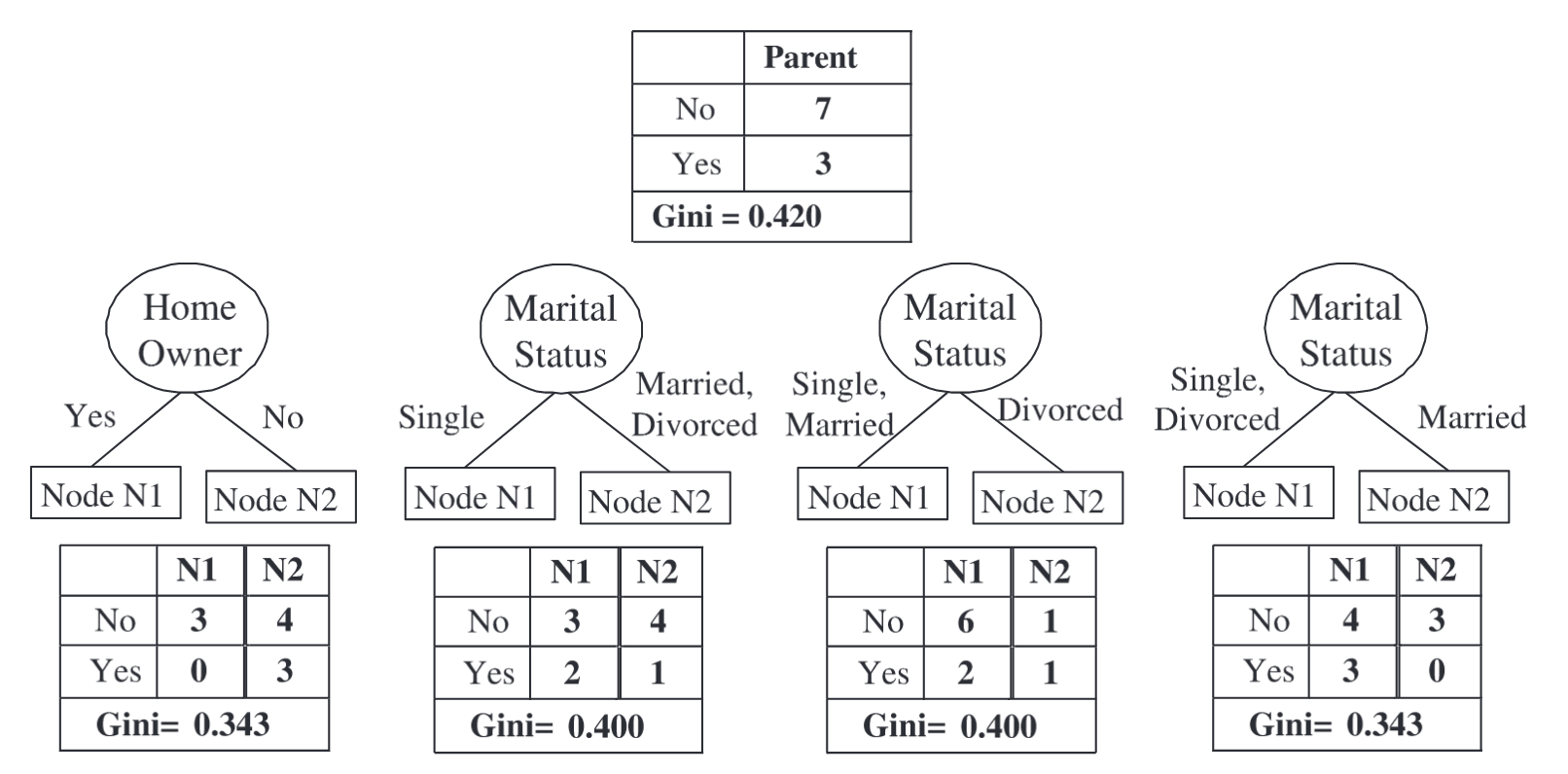
Here’s an example of how to identify the best attribute test condition using the Collective Impurity of the Gini Impurity index.
Code
def gini_impurity(yes_count, no_count):
    """Calculate Gini impurity for a node"""
    total = yes_count + no_count
    if total == 0:
        return 0

    p_yes = yes_count / total
    p_no = no_count / total

    gini = 1 - (p_yes**2 + p_no**2)
    return gini

def weighted_gini(n1_yes, n1_no, n2_yes, n2_no):
    """Calculate weighted average Gini impurity after split"""
    n1_total = n1_yes + n1_no
    n2_total = n2_yes + n2_no
    total = n1_total + n2_total

    gini_n1 = gini_impurity(n1_yes, n1_no)
    gini_n2 = gini_impurity(n2_yes, n2_no)

    weighted_gini = (n1_total/total) * gini_n1 + (n2_total/total) * gini_n2
    return weighted_gini

# Parent node
parent_yes = 3
parent_no = 7
parent_gini = gini_impurity(parent_yes, parent_no)

print("=" * 60)
print("PARENT NODE")
print("=" * 60)
print(f"Yes: {parent_yes}, No: {parent_no}")
print(f"Gini Impurity: {parent_gini:.3f}")
print()

# Define all four splits
splits = {
    "Home Owner": {
        "N1": {"yes": 0, "no": 3},  # Yes (owns home)
        "N2": {"yes": 3, "no": 4}   # No (doesn't own home)
    },
    "Marital Status (Split 1: Single vs Married+Divorced)": {
        "N1": {"yes": 2, "no": 3},  # Single
        "N2": {"yes": 1, "no": 4}   # Married, Divorced
    },
    "Marital Status (Split 2: Single+Married vs Divorced)": {
        "N1": {"yes": 2, "no": 6},  # Single, Married
        "N2": {"yes": 1, "no": 1}   # Divorced
    },
    "Marital Status (Split 3: Single+Divorced vs Married)": {
        "N1": {"yes": 3, "no": 4},  # Single, Divorced
        "N2": {"yes": 0, "no": 3}   # Married
    }
}

# Calculate for each split
results = []
for split_name, nodes in splits.items():
    n1_yes = nodes["N1"]["yes"]
    n1_no = nodes["N1"]["no"]
    n2_yes = nodes["N2"]["yes"]
    n2_no = nodes["N2"]["no"]

    gini_n1 = gini_impurity(n1_yes, n1_no)
    gini_n2 = gini_impurity(n2_yes, n2_no)
    weighted_gini_value = weighted_gini(n1_yes, n1_no, n2_yes, n2_no)
    gini_gain = parent_gini - weighted_gini_value

    results.append({
        'name': split_name,
        'weighted_gini': weighted_gini_value,
        'gini_gain': gini_gain,
        'gini_n1': gini_n1,
        'gini_n2': gini_n2,
        'n1_yes': n1_yes,
        'n1_no': n1_no,
        'n2_yes': n2_yes,
        'n2_no': n2_no
    })

    print("=" * 60)
    print(f"SPLIT: {split_name}")
    print("=" * 60)
    print(f"Node N1: Yes={n1_yes}, No={n1_no}, Total={n1_yes+n1_no}")
    print(f"  Gini(N1) = {gini_n1:.3f}")
    print(f"Node N2: Yes={n2_yes}, No={n2_no}, Total={n2_yes+n2_no}")
    print(f"  Gini(N2) = {gini_n2:.3f}")
    print(f"\nWeighted Gini (after split): {weighted_gini_value:.3f}")
    print(f"Gini Gain: {gini_gain:.3f}")
    print()

# Summary: Find best split
print("=" * 60)
print("SUMMARY - BEST SPLIT")
print("=" * 60)
results_sorted = sorted(results, key=lambda x: x['gini_gain'], reverse=True)
for i, result in enumerate(results_sorted, 1):
    print(f"{i}. {result['name']}")
    print(f"   Weighted Gini: {result['weighted_gini']:.3f}, Gini Gain: {result['gini_gain']:.3f}")
print()
print(f"Best split: {results_sorted[0]['name']}")
print(f"Maximum Gini Gain: {results_sorted[0]['gini_gain']:.3f}")
============================================================
PARENT NODE
============================================================
Yes: 3, No: 7
Gini Impurity: 0.420
============================================================
SPLIT: Home Owner
============================================================
Node N1: Yes=0, No=3, Total=3
Gini(N1) = 0.000
Node N2: Yes=3, No=4, Total=7
Gini(N2) = 0.490
Weighted Gini (after split): 0.343
Gini Gain: 0.077
============================================================
SPLIT: Marital Status (Split 1: Single vs Married+Divorced)
============================================================
Node N1: Yes=2, No=3, Total=5
Gini(N1) = 0.480
Node N2: Yes=1, No=4, Total=5
Gini(N2) = 0.320
Weighted Gini (after split): 0.400
Gini Gain: 0.020
============================================================
SPLIT: Marital Status (Split 2: Single+Married vs Divorced)
============================================================
Node N1: Yes=2, No=6, Total=8
Gini(N1) = 0.375
Node N2: Yes=1, No=1, Total=2
Gini(N2) = 0.500
Weighted Gini (after split): 0.400
Gini Gain: 0.020
============================================================
SPLIT: Marital Status (Split 3: Single+Divorced vs Married)
============================================================
Node N1: Yes=3, No=4, Total=7
Gini(N1) = 0.490
Node N2: Yes=0, No=3, Total=3
Gini(N2) = 0.000
Weighted Gini (after split): 0.343
Gini Gain: 0.077
============================================================
SUMMARY - BEST SPLIT
============================================================
1. Home Owner
Weighted Gini: 0.343, Gini Gain: 0.077
2. Marital Status (Split 3: Single+Divorced vs Married)
Weighted Gini: 0.343, Gini Gain: 0.077
3. Marital Status (Split 1: Single vs Married+Divorced)
Weighted Gini: 0.400, Gini Gain: 0.020
4. Marital Status (Split 2: Single+Married vs Divorced)
Weighted Gini: 0.400, Gini Gain: 0.020
Best split: Home Owner
Maximum Gini Gain: 0.077Splitting Continuous Attributes
For quantitative attributes like Annual Income, we need to find some threshold \(\tau\) that minimizes the impurity index.
The following table illustrates the process.
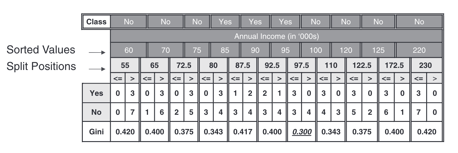
Procedure:
- Sort all the training instances by Annual Income in increasing order.
- Pick thresholds half way between consecutive values.
- Compute the Gini impurity index for each threshold.
- Select the threshold that minimizes the Gini impurity index.
Code
def gini_impurity(yes_count, no_count):
    """Calculate Gini impurity for a node"""
    total = yes_count + no_count
    if total == 0:
        return 0

    p_yes = yes_count / total
    p_no = no_count / total

    gini = 1 - (p_yes**2 + p_no**2)
    return gini

def weighted_gini_split(left_yes, left_no, right_yes, right_no):
    """Calculate weighted Gini impurity for a binary split"""
    left_total = left_yes + left_no
    right_total = right_yes + right_no
    total = left_total + right_total

    if total == 0:
        return 0

    gini_left = gini_impurity(left_yes, left_no)
    gini_right = gini_impurity(right_yes, right_no)

    weighted_gini = (left_total/total) * gini_left + (right_total/total) * gini_right
    return weighted_gini

# Data from the table
sorted_values = [60, 70, 75, 85, 90, 95, 100, 120, 125, 220]
classes = ['No', 'No', 'No', 'Yes', 'Yes', 'Yes', 'No', 'No', 'No', 'No']

# Calculate split positions (midpoints between consecutive values)
split_positions = []
for i in range(len(sorted_values) - 1):
    split_pos = (sorted_values[i] + sorted_values[i+1]) / 2
    split_positions.append(split_pos)

# Parent node statistics
parent_yes = classes.count('Yes')
parent_no = classes.count('No')
parent_gini = gini_impurity(parent_yes, parent_no)

print("=" * 80)
print("CONTINUOUS ATTRIBUTE: Annual Income")
print("=" * 80)
print(f"Parent Node: Yes={parent_yes}, No={parent_no}")
print(f"Parent Gini Impurity: {parent_gini:.3f}")
print()

print("=" * 80)
print("EVALUATING ALL POSSIBLE SPLITS")
print("=" * 80)

best_split = None
best_gini = float('inf')
best_gain = -float('inf')

results = []

for i, split_pos in enumerate(split_positions):
    # Count classes on left (<= split) and right (> split)
    left_yes = 0
    left_no = 0
    right_yes = 0
    right_no = 0

    for j, value in enumerate(sorted_values):
        if value <= split_pos:
            if classes[j] == 'Yes':
                left_yes += 1
            else:
                left_no += 1
        else:
            if classes[j] == 'Yes':
                right_yes += 1
            else:
                right_no += 1

    # Calculate weighted Gini
    weighted_gini = weighted_gini_split(left_yes, left_no, right_yes, right_no)
    gini_gain = parent_gini - weighted_gini

    results.append({
        'split_position': split_pos,
        'left_yes': left_yes,
        'left_no': left_no,
        'right_yes': right_yes,
        'right_no': right_no,
        'weighted_gini': weighted_gini,
        'gini_gain': gini_gain
    })

    print(f"Split at {split_pos:6.1f}:")
    print(f"  Left  (<=): Yes={left_yes}, No={left_no}, Total={left_yes+left_no}")
    print(f"  Right ( >): Yes={right_yes}, No={right_no}, Total={right_yes+right_no}")
    print(f"  Weighted Gini: {weighted_gini:.3f}")
    print(f"  Gini Gain: {gini_gain:.3f}")

    if weighted_gini < best_gini:
        best_gini = weighted_gini
        best_split = split_pos
        best_gain = gini_gain

    print()

print("=" * 80)
print("BEST SPLIT")
print("=" * 80)
print(f"Best Split Position: {best_split}")
print(f"Minimum Weighted Gini: {best_gini:.3f}")
print(f"Maximum Gini Gain: {best_gain:.3f}")

# Show the split details
best_result = [r for r in results if r['split_position'] == best_split][0]
print(f"\nSplit Details (Annual Income <= {best_split}):")
print(f"  Left  (<=): Yes={best_result['left_yes']}, No={best_result['left_no']}")
print(f"  Right ( >): Yes={best_result['right_yes']}, No={best_result['right_no']}")
================================================================================
CONTINUOUS ATTRIBUTE: Annual Income
================================================================================
Parent Node: Yes=3, No=7
Parent Gini Impurity: 0.420
================================================================================
EVALUATING ALL POSSIBLE SPLITS
================================================================================
Split at 65.0:
Left (<=): Yes=0, No=1, Total=1
Right ( >): Yes=3, No=6, Total=9
Weighted Gini: 0.400
Gini Gain: 0.020
Split at 72.5:
Left (<=): Yes=0, No=2, Total=2
Right ( >): Yes=3, No=5, Total=8
Weighted Gini: 0.375
Gini Gain: 0.045
Split at 80.0:
Left (<=): Yes=0, No=3, Total=3
Right ( >): Yes=3, No=4, Total=7
Weighted Gini: 0.343
Gini Gain: 0.077
Split at 87.5:
Left (<=): Yes=1, No=3, Total=4
Right ( >): Yes=2, No=4, Total=6
Weighted Gini: 0.417
Gini Gain: 0.003
Split at 92.5:
Left (<=): Yes=2, No=3, Total=5
Right ( >): Yes=1, No=4, Total=5
Weighted Gini: 0.400
Gini Gain: 0.020
Split at 97.5:
Left (<=): Yes=3, No=3, Total=6
Right ( >): Yes=0, No=4, Total=4
Weighted Gini: 0.300
Gini Gain: 0.120
Split at 110.0:
Left (<=): Yes=3, No=4, Total=7
Right ( >): Yes=0, No=3, Total=3
Weighted Gini: 0.343
Gini Gain: 0.077
Split at 122.5:
Left (<=): Yes=3, No=5, Total=8
Right ( >): Yes=0, No=2, Total=2
Weighted Gini: 0.375
Gini Gain: 0.045
Split at 172.5:
Left (<=): Yes=3, No=6, Total=9
Right ( >): Yes=0, No=1, Total=1
Weighted Gini: 0.400
Gini Gain: 0.020
================================================================================
BEST SPLIT
================================================================================
Best Split Position: 97.5
Minimum Weighted Gini: 0.300
Maximum Gini Gain: 0.120
Split Details (Annual Income <= 97.5):
Left (<=): Yes=3, No=3
Right ( >): Yes=0, No=4Run Decision Tree on Loans Data Set
Let’s run the Scikit-learn Decision Tree, sklearn.tree, on the loans data set.
sklearn.tree requires all fields to be numeric.
So first we have to convert the categorical fields to category index numeric fields.
loans['Defaulted Borrower'] = loans['Defaulted Borrower'].cat.codes
loans['Home Owner'] = loans['Home Owner'].cat.codes
loans['Marital Status'] = loans['Marital Status'].cat.codes
loans.head()| Home Owner | Marital Status | Annual Income | Defaulted Borrower | |
|---|---|---|---|---|
| ID | ||||
| 1 | 1 | 2 | 125000 | 0 |
| 2 | 0 | 1 | 100000 | 0 |
| 3 | 0 | 2 | 70000 | 0 |
| 4 | 1 | 1 | 120000 | 0 |
| 5 | 0 | 0 | 95000 | 1 |
Then the independent variables are all the fields except the “Defaulted Borrower” field, which we’ll assign to X.
The dependent variable is the “Defaulted Borrower” field, which we’ll assign to y.
from sklearn import tree

X = loans.drop('Defaulted Borrower', axis=1)
y = loans['Defaulted Borrower']X:
<class 'pandas.core.frame.DataFrame'>
Index: 10 entries, 1 to 10
Data columns (total 3 columns):
 #   Column          Non-Null Count  Dtype
---  ------          --------------  -----
 0   Home Owner      10 non-null     int8
 1   Marital Status  10 non-null     int8
 2   Annual Income   10 non-null     int64
dtypes: int64(1), int8(2)
memory usage: 180.0 bytesy:
<class 'pandas.core.series.Series'>
Index: 10 entries, 1 to 10
Series name: Defaulted Borrower
Non-Null Count  Dtype
--------------  -----
10 non-null     int8
dtypes: int8(1)
memory usage: 90.0 bytes
Let’s fit a decision tree to the data.
clf = tree.DecisionTreeClassifier(criterion='gini', random_state=42)
clf = clf.fit(X, y)
Let’s plot the tree.
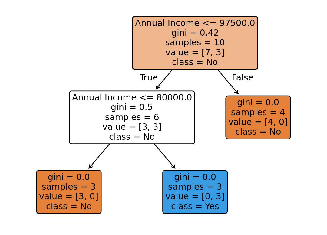
Interestingly, the tree was built using only the Income field.
That’s arguably an advantage of Decision Trees: they automatically perform feature selection.
Ensemble Methods
(See Tan et al. (2018), Chapter 4)
Motivated around the idea that combining several noisy classifiers can result in a better prediction under certain conditions.
- The base classifiers are independent
- The base classifiers are noisy (high variance)
- The base classifiers are low (ideally zero) bias
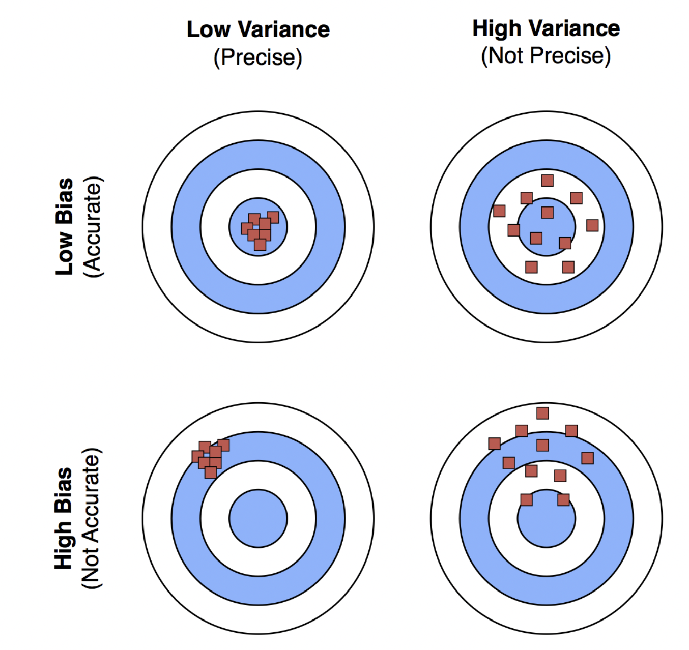
Bias and Variance
Bias
- Definition: Error due to overly simplistic models.
- High bias: Model underfits the data.
- Example: Shallow decision trees.
- Low bias: Model accurately captures the underlying patterns in the data.
- Example: Deep decision trees.
Variance
- Definition: Error due to overly complex models.
- High Variance: Model overfits the data.
- Example: Deep decision trees.
- Low variance: Model predictions are stable and consistent across different training datasets.
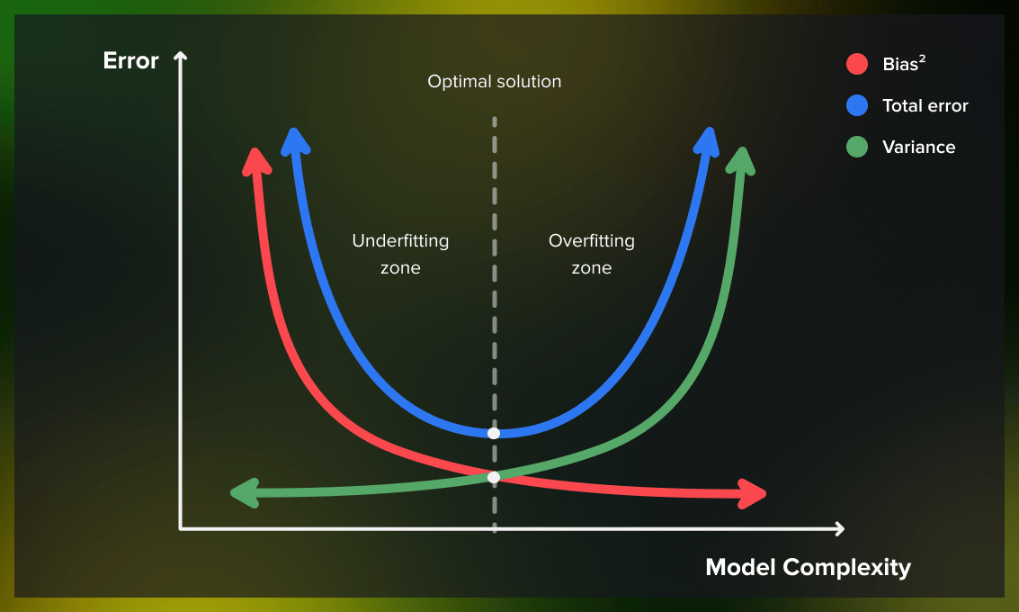
Bias Variance Trade-Off
Goal: Find a balance to minimize total error.
Bias-Variance Trade-off: Low bias and low variance are ideal but challenging to achieve simultaneously.
Random Forests
Random forests are an ensemble of decision trees that:
- Construct a set of base classifiers from random sub-samples of the training data.
- Train each base classifier to completion.
- Take a majority vote of the base classifiers to form the final prediction.
Titanic Example
We’ll use the Titanic data set and excerpts of this Kaggle tutorial to illustrate the concepts of overfitting and random forests.
Code
import pandas as pd

import os
import urllib.request

# Check if the directory exists, if not, create it
if not os.path.exists('data/titanic'):
    os.makedirs('data/titanic')

if not os.path.exists('data/titanic/train.csv'):
    url = 'https://raw.githubusercontent.com/tools4ds/DS701-Course-Notes/refs/heads/main/ds701_book/data/titanic/train.csv'
    urllib.request.urlretrieve(url, 'data/titanic/train.csv')

df_train = pd.read_csv('data/titanic/train.csv', index_col='PassengerId')

if not os.path.exists('data/titanic/test.csv'):
    url = 'https://raw.githubusercontent.com/tools4ds/DS701-Course-Notes/refs/heads/main/ds701_book/data/titanic/test.csv'
    urllib.request.urlretrieve(url, 'data/titanic/test.csv')

df_test = pd.read_csv('data/titanic/test.csv', index_col='PassengerId')
Let’s look at the training data.
Code
df_train.info()<class 'pandas.core.frame.DataFrame'>
Index: 891 entries, 1 to 891
Data columns (total 11 columns):
# Column Non-Null Count Dtype
--- ------ -------------- -----
0 Survived 891 non-null int64
1 Pclass 891 non-null int64
2 Name 891 non-null object
3 Sex 891 non-null object
4 Age 714 non-null float64
5 SibSp 891 non-null int64
6 Parch 891 non-null int64
7 Ticket 891 non-null object
8 Fare 891 non-null float64
9 Cabin 204 non-null object
10 Embarked 889 non-null object
dtypes: float64(2), int64(4), object(5)
memory usage: 83.5+ KBWe can see that there are 891 entries with 11 fields. ‘Age’, ‘Cabin’, and ‘Embarked’ have missing values.
Code
df_train.head()| Survived | Pclass | Name | Sex | Age | SibSp | Parch | Ticket | Fare | Cabin | Embarked | |
|---|---|---|---|---|---|---|---|---|---|---|---|
| PassengerId | |||||||||||
| 1 | 0 | 3 | Braund, Mr. Owen Harris | male | 22.0 | 1 | 0 | A/5 21171 | 7.2500 | NaN | S |
| 2 | 1 | 1 | Cumings, Mrs. John Bradley (Florence Briggs Th... | female | 38.0 | 1 | 0 | PC 17599 | 71.2833 | C85 | C |
| 3 | 1 | 3 | Heikkinen, Miss. Laina | female | 26.0 | 0 | 0 | STON/O2. 3101282 | 7.9250 | NaN | S |
| 4 | 1 | 1 | Futrelle, Mrs. Jacques Heath (Lily May Peel) | female | 35.0 | 1 | 0 | 113803 | 53.1000 | C123 | S |
| 5 | 0 | 3 | Allen, Mr. William Henry | male | 35.0 | 0 | 0 | 373450 | 8.0500 | NaN | S |
Let’s look at the test data.
Code
df_test.info()
df_test.head()
<class 'pandas.core.frame.DataFrame'>
Index: 418 entries, 892 to 1309
Data columns (total 10 columns):
# Column Non-Null Count Dtype
--- ------ -------------- -----
0 Pclass 418 non-null int64
1 Name 418 non-null object
2 Sex 418 non-null object
3 Age 332 non-null float64
4 SibSp 418 non-null int64
5 Parch 418 non-null int64
6 Ticket 418 non-null object
7 Fare 417 non-null float64
8 Cabin 91 non-null object
9 Embarked 418 non-null object
dtypes: float64(2), int64(3), object(5)
memory usage: 35.9+ KB| Pclass | Name | Sex | Age | SibSp | Parch | Ticket | Fare | Cabin | Embarked | |
|---|---|---|---|---|---|---|---|---|---|---|
| PassengerId | ||||||||||
| 892 | 3 | Kelly, Mr. James | male | 34.5 | 0 | 0 | 330911 | 7.8292 | NaN | Q |
| 893 | 3 | Wilkes, Mrs. James (Ellen Needs) | female | 47.0 | 1 | 0 | 363272 | 7.0000 | NaN | S |
| 894 | 2 | Myles, Mr. Thomas Francis | male | 62.0 | 0 | 0 | 240276 | 9.6875 | NaN | Q |
| 895 | 3 | Wirz, Mr. Albert | male | 27.0 | 0 | 0 | 315154 | 8.6625 | NaN | S |
| 896 | 3 | Hirvonen, Mrs. Alexander (Helga E Lindqvist) | female | 22.0 | 1 | 1 | 3101298 | 12.2875 | NaN | S |
There are 418 entries in the test set with same fields except for ‘Survived’, which is what we need to predict.
We’ll do some data cleaning and preparation.
Code
import numpy as np

def proc_data(df):
    df['Fare'] = df.Fare.fillna(0)
    df.fillna(modes, inplace=True) # Fill missing values with the mode
    df['LogFare'] = np.log1p(df['Fare'])  # Create a new column for the log of the fare + 1
    df['Embarked'] = pd.Categorical(df.Embarked)  # Convert to categorical
    df['Sex'] = pd.Categorical(df.Sex)  # Convert to categorical

modes = df_train.mode().iloc[0] # Get the mode for each column

proc_data(df_train)
proc_data(df_test)
Look at the dataframes again.
Code
df_train.info()<class 'pandas.core.frame.DataFrame'>
Index: 891 entries, 1 to 891
Data columns (total 12 columns):
# Column Non-Null Count Dtype
--- ------ -------------- -----
0 Survived 891 non-null int64
1 Pclass 891 non-null int64
2 Name 891 non-null object
3 Sex 891 non-null category
4 Age 891 non-null float64
5 SibSp 891 non-null int64
6 Parch 891 non-null int64
7 Ticket 891 non-null object
8 Fare 891 non-null float64
9 Cabin 891 non-null object
10 Embarked 891 non-null category
11 LogFare 891 non-null float64
dtypes: category(2), float64(3), int64(4), object(3)
memory usage: 78.6+ KBCode
df_test.info()<class 'pandas.core.frame.DataFrame'>
Index: 418 entries, 892 to 1309
Data columns (total 11 columns):
# Column Non-Null Count Dtype
--- ------ -------------- -----
0 Pclass 418 non-null int64
1 Name 418 non-null object
2 Sex 418 non-null category
3 Age 418 non-null float64
4 SibSp 418 non-null int64
5 Parch 418 non-null int64
6 Ticket 418 non-null object
7 Fare 418 non-null float64
8 Cabin 418 non-null object
9 Embarked 418 non-null category
10 LogFare 418 non-null float64
dtypes: category(2), float64(3), int64(3), object(3)
memory usage: 33.7+ KBWe’ll create lists of features by type.
cats=["Sex","Embarked"]  # Categorical
conts=['Age', 'SibSp', 'Parch', 'LogFare',"Pclass"]  # Continuous
dep="Survived"  # Dependent variable
Let’s explore some fields starting with survival rate by gender.
Code
import seaborn as sns
import matplotlib.pyplot as plt
fig,axs = plt.subplots(1,2, figsize=(11,5))
sns.barplot(data=df_train, y='Survived', x="Sex", ax=axs[0], hue="Sex", palette=["#3374a1","#e1812d"]).set(title="Survival rate")
sns.countplot(data=df_train, x="Sex", ax=axs[1], hue="Sex", palette=["#3374a1","#e1812d"]).set(title="Histogram");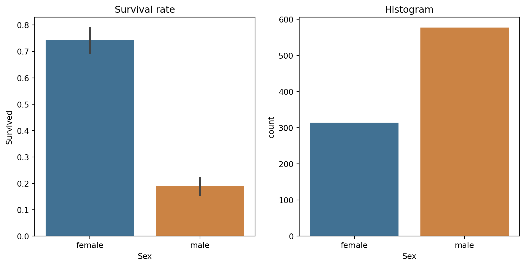
Indeed, “women and children first” was enforced on the Titanic.
Since we don’t have labels for the test data, we’ll split the training data into training and validation.
from numpy import random
from sklearn.model_selection import train_test_split

random.seed(42)
trn_df,val_df = train_test_split(df_train, test_size=0.25)

# Replace categorical fields with numeric codes
trn_df[cats] = trn_df[cats].apply(lambda x: x.cat.codes)
val_df[cats] = val_df[cats].apply(lambda x: x.cat.codes)
Let’s split the independent (input) variables from the dependent (output) variable.
def xs_y(df):
    xs = df[cats+conts].copy()
    return xs,df[dep] if dep in df else None

trn_xs,trn_y = xs_y(trn_df)
val_xs,val_y = xs_y(val_df)
Here’s the predictions for our extremely simple model, where female is coded as 0:
preds = val_xs.Sex==0We’ll use mean absolute error to measure how good this model is:
from sklearn.metrics import mean_absolute_error
mean_absolute_error(val_y, preds)0.21524663677130046Alternatively, we could try splitting on a continuous column. We have to use a somewhat different chart to see how this might work – here’s an example of how we could look at LogFare:
Code
df_fare = trn_df[trn_df.LogFare>0]
fig,axs = plt.subplots(1,2, figsize=(11,5))
sns.boxenplot(data=df_fare, x=dep, y="LogFare", ax=axs[0], hue=dep, palette=["#3374a1","#e1812d"])
sns.kdeplot(data=df_fare, x="LogFare", ax=axs[1]);
The boxenplot above shows quantiles of LogFare for each group of Survived==0 and Survived==1.
It shows that the average LogFare for passengers that didn’t survive is around 2.5, and for those that did it’s around 3.2.
So it seems that people that paid more for their tickets were more likely to get put on a lifeboat.
Let’s create a simple model based on this observation:
preds = val_xs.LogFare>2.7…and test it out:
mean_absolute_error(val_y, preds)0.336322869955157This is quite a bit less accurate than our model that used Sex as the single binary split.
Full Decision Tree
Ok. Let’s build a decision tree model using all the features.
clf = tree.DecisionTreeClassifier(criterion='gini', random_state=42)
clf = clf.fit(trn_xs, trn_y)
Let’s draw the tree.
annotations = tree.plot_tree(clf,
               filled=True,
               rounded=True,
               feature_names=trn_xs.columns,
               class_names=['No', 'Yes'])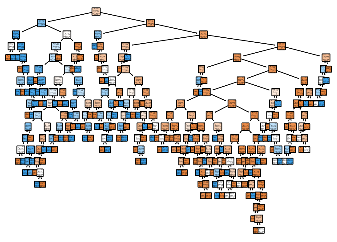
Full Tree – Evaluation Error
Let’s see how it does on the validation set.
preds = clf.predict(val_xs)
mean_absolute_error(val_y, preds)0.2645739910313901That is quite a bit worse than splitting on Sex alone!!
Stopping Criteria – Minimum Samples Split
Let’s train the decision tree again but with stopping criteria based on the number of samples in a node.
clf = tree.DecisionTreeClassifier(criterion='gini', random_state=42, min_samples_split=20)
clf = clf.fit(trn_xs, trn_y)
Let’s draw the tree.
annotations = tree.plot_tree(clf,
               filled=True,
               rounded=True,
               feature_names=trn_xs.columns,
               class_names=['No', 'Yes'])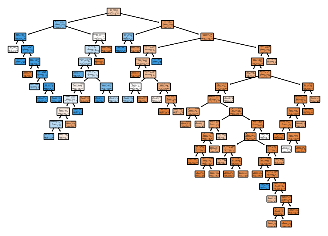
Min Samples Split – Evaluation Error
Let’s see how it does on the validation set.
preds = clf.predict(val_xs)
mean_absolute_error(val_y, preds)0.18834080717488788Decision Tree – Maximum Depth
Let’s train the decision tree again but with a maximum depth of 3.
clf = tree.DecisionTreeClassifier(criterion='gini', random_state=42, max_depth=3)
clf = clf.fit(trn_xs, trn_y)
Let’s draw the tree.
annotations = tree.plot_tree(clf,
               filled=True,
               rounded=True,
               feature_names=trn_xs.columns,
               class_names=['No', 'Yes'])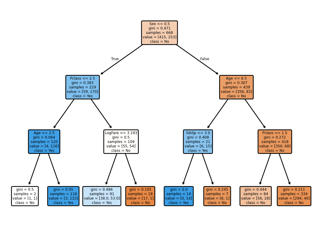
Maximum Depth – Evaluation Error
Let’s see how it does on the validation set.
preds = clf.predict(val_xs)
mean_absolute_error(val_y, preds)0.19730941704035873Random Forest
Let’s try a random forest.
from sklearn.ensemble import RandomForestClassifier

clf = RandomForestClassifier(n_estimators=100, random_state=42)
clf = clf.fit(trn_xs, trn_y)
Let’s see how it does on the validation set.
preds = clf.predict(val_xs)
mean_absolute_error(val_y, preds)0.21076233183856502References
Hastie, Trevor, Robert Tibshirani, and Jerome Friedman. 2009. The Elements of Statistical Learning. 2nd ed. Springer. https://hastie.su.domains/ElemStatLearn/.
Tan, Pang-Ning, Michael Steinbach, and Vipin Kumar. 2018. Introduction to Data Mining. 2nd ed. Pearson. https://www-users.cse.umn.edu/~kumar001/dmbook/ch3_classification.pdf.