Code
import numpy as np
import matplotlib.pyplot as plt
import pandas as pd
import seaborn as sns
from IPython.display import Image, HTML
import warnings
warnings.filterwarnings('ignore')

%matplotlib inline![]()
import numpy as np
import matplotlib.pyplot as plt
import pandas as pd
import seaborn as sns
from IPython.display import Image, HTML
import warnings
warnings.filterwarnings('ignore')
%matplotlib inlineIn previous lectures, we built neural networks from scratch and used PyTorch. Now we’ll explore scikit-learn’s neural network capabilities, which provide a simpler, high-level interface for many common tasks.
While PyTorch and TensorFlow are more powerful for complex deep learning tasks, scikit-learn’s MLPClassifier and MLPRegressor are excellent for:
Scikit-learn provides two main classes for neural networks:
MLPClassifier: Multi-layer Perceptron classifierMLPRegressor: Multi-layer Perceptron regressorBoth use the same underlying architecture but differ in their output layer and loss function.
Key features:
'relu', 'tanh', 'logistic', 'identity''adam', 'sgd', 'lbfgs'alphaThe architecture is specified as a tuple of hidden layer sizes:
# Single hidden layer with 100 neurons
hidden_layer_sizes=(100,)

# Two hidden layers with 100 and 50 neurons
hidden_layer_sizes=(100, 50)

# Three hidden layers
hidden_layer_sizes=(128, 64, 32)
The input and output layers are automatically determined from the data.
Let’s classify handwritten digits using the MNIST dataset.
from sklearn.datasets import fetch_openml
from sklearn.model_selection import train_test_split
from sklearn.preprocessing import StandardScaler

# Load MNIST data (this may take a moment)
print("Loading MNIST dataset...")
X, y = fetch_openml('mnist_784', version=1, return_X_y=True, as_frame=False, parser='auto')

# Convert labels to integers (they come as strings from fetch_openml)
y = y.astype(int)

# Use a subset for faster training in this demo
# Remove this line to use the full dataset
X, _, y, _ = train_test_split(X, y, train_size=10000, stratify=y, random_state=42)

print(f"Dataset shape: {X.shape}")
print(f"Number of classes: {len(np.unique(y))}")
print(f"Label type: {y.dtype}")
Loading MNIST dataset...
Dataset shape: (10000, 784)
Number of classes: 10
Label type: int64Split into training and test sets:
# Split the data
X_train, X_test, y_train, y_test = train_test_split(
    X, y, test_size=0.2, random_state=42
)

print(f"Training set size: {X_train.shape[0]}")
print(f"Test set size: {X_test.shape[0]}")
Training set size: 8000
Test set size: 2000Visualize some examples:
fig, axes = plt.subplots(2, 5, figsize=(12, 5))
for i, ax in enumerate(axes.flat):
    ax.imshow(X_train[i].reshape(28, 28), cmap='gray')
    ax.set_title(f'Label: {y_train[i]}')
    ax.axis('off')
plt.tight_layout()
plt.show()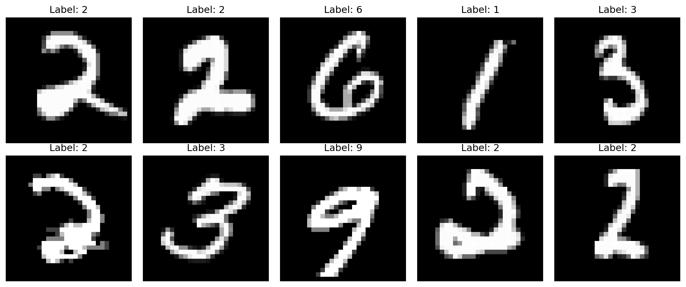
Neural networks work best with normalized data:
# Scale features to [0, 1] range (pixels are already in [0, 255])
X_train_scaled = X_train / 255.0
X_test_scaled = X_test / 255.0

print(f"Feature range: [{X_train_scaled.min():.2f}, {X_train_scaled.max():.2f}]")
Feature range: [0.00, 1.00]Alternatively, you could use StandardScaler() to normalize to zero mean and unit variance, which is often preferred for neural networks.
from sklearn.neural_network import MLPClassifier

# Create MLP with 2 hidden layers
mlp = MLPClassifier(
    hidden_layer_sizes=(128, 64),  # Two hidden layers
    activation='relu',              # ReLU activation
    solver='adam',                  # Adam optimizer
    alpha=0.0001,                   # L2 regularization
    batch_size=64,                  # Mini-batch size
    learning_rate_init=0.001,       # Initial learning rate
    max_iter=20,                    # Number of epochs
    random_state=42,
    verbose=True                    # Print progress
)

# Train the model
print("Training MLP...")
mlp.fit(X_train_scaled, y_train)
Training MLP...
Iteration 1, loss = 0.71345206
Iteration 2, loss = 0.26439384
Iteration 3, loss = 0.18880844
Iteration 4, loss = 0.14070827
Iteration 5, loss = 0.10813206
Iteration 6, loss = 0.08241134
Iteration 7, loss = 0.06312883
Iteration 8, loss = 0.04742022
Iteration 9, loss = 0.03751731
Iteration 10, loss = 0.02680532
Iteration 11, loss = 0.02321482
Iteration 12, loss = 0.01516949
Iteration 13, loss = 0.01235069
Iteration 14, loss = 0.00823132
Iteration 15, loss = 0.00665425
Iteration 16, loss = 0.00515634
Iteration 17, loss = 0.00431783
Iteration 18, loss = 0.00336489
Iteration 19, loss = 0.00283319
Iteration 20, loss = 0.00253876MLPClassifier(batch_size=64, hidden_layer_sizes=(128, 64), max_iter=20,
random_state=42, verbose=True)In a Jupyter environment, please rerun this cell to show the HTML representation or trust the notebook. MLPClassifier(batch_size=64, hidden_layer_sizes=(128, 64), max_iter=20,
random_state=42, verbose=True)The verbose=True parameter shows the loss at each iteration, similar to what we saw in our custom implementation and PyTorch.
from sklearn.metrics import accuracy_score, classification_report, confusion_matrix

# Make predictions
y_pred = mlp.predict(X_test_scaled)

# Calculate accuracy
accuracy = accuracy_score(y_test, y_pred)
print(f"\nTest Accuracy: {accuracy:.4f}")
Test Accuracy: 0.9555Detailed classification report:
print("\nClassification Report:")
print(classification_report(y_test, y_pred))
Classification Report:
              precision    recall  f1-score   support

           0       0.95      0.99      0.97       191
           1       0.98      1.00      0.99       226
           2       0.94      0.96      0.95       215
           3       0.95      0.93      0.94       202
           4       0.98      0.94      0.96       206
           5       0.96      0.94      0.95       168
           6       0.98      0.97      0.98       196
           7       0.93      0.96      0.95       185
           8       0.96      0.95      0.95       206
           9       0.91      0.91      0.91       205

    accuracy                           0.96      2000
   macro avg       0.96      0.96      0.96      2000
weighted avg       0.96      0.96      0.96      2000
Visualize the confusion matrix:
from sklearn.metrics import ConfusionMatrixDisplay

fig, ax = plt.subplots(figsize=(10, 8))
cm = confusion_matrix(y_test, y_pred)
disp = ConfusionMatrixDisplay(confusion_matrix=cm, display_labels=mlp.classes_)
disp.plot(ax=ax, cmap='Blues', values_format='d')
plt.title('Confusion Matrix for MNIST Classification')
plt.show()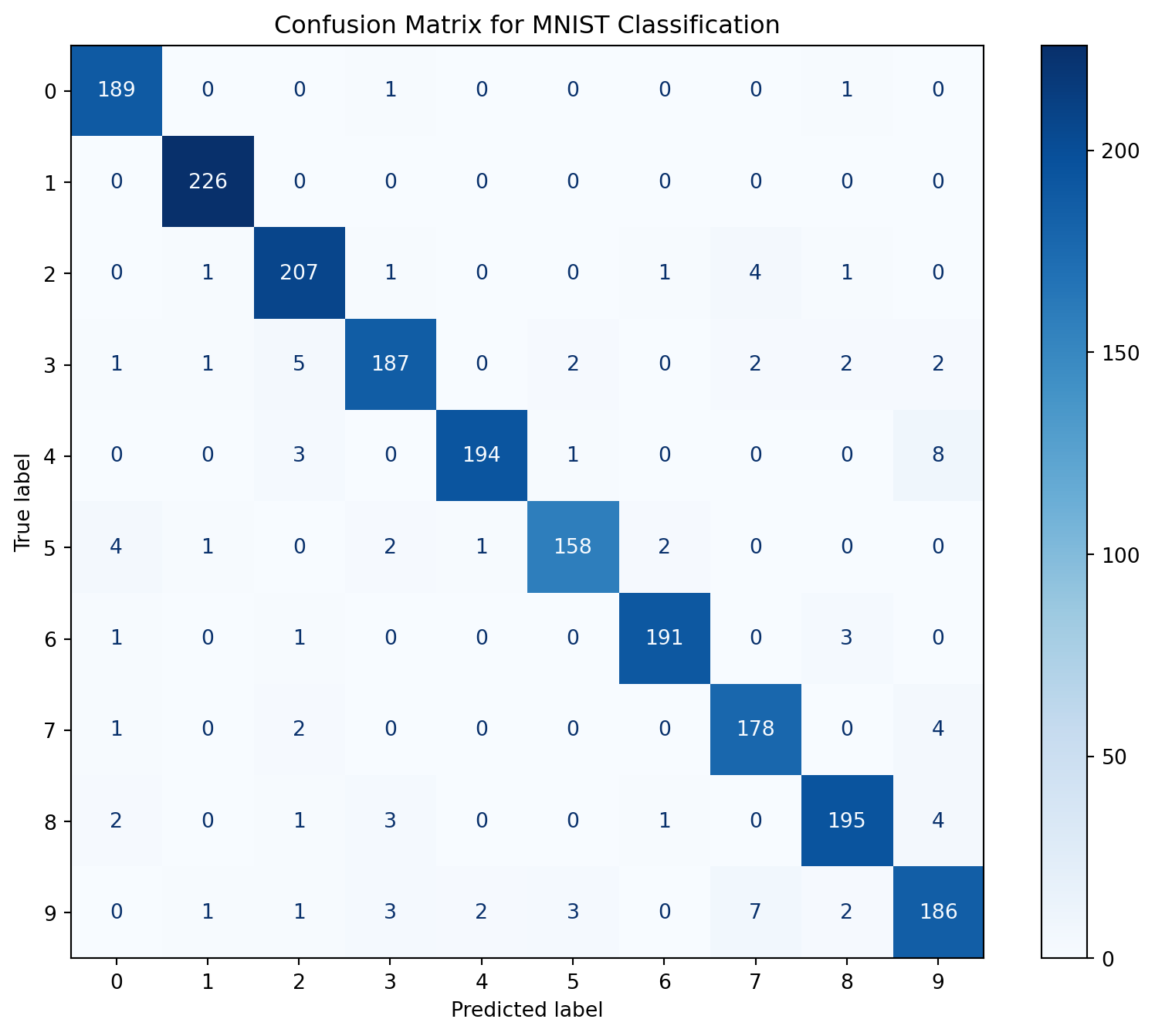
Scikit-learn’s MLP stores the loss at each iteration:
plt.figure(figsize=(10, 6))
plt.plot(mlp.loss_curve_)
plt.xlabel('Iteration')
plt.ylabel('Loss')
plt.title('Training Loss Curve')
plt.grid(True)
plt.show()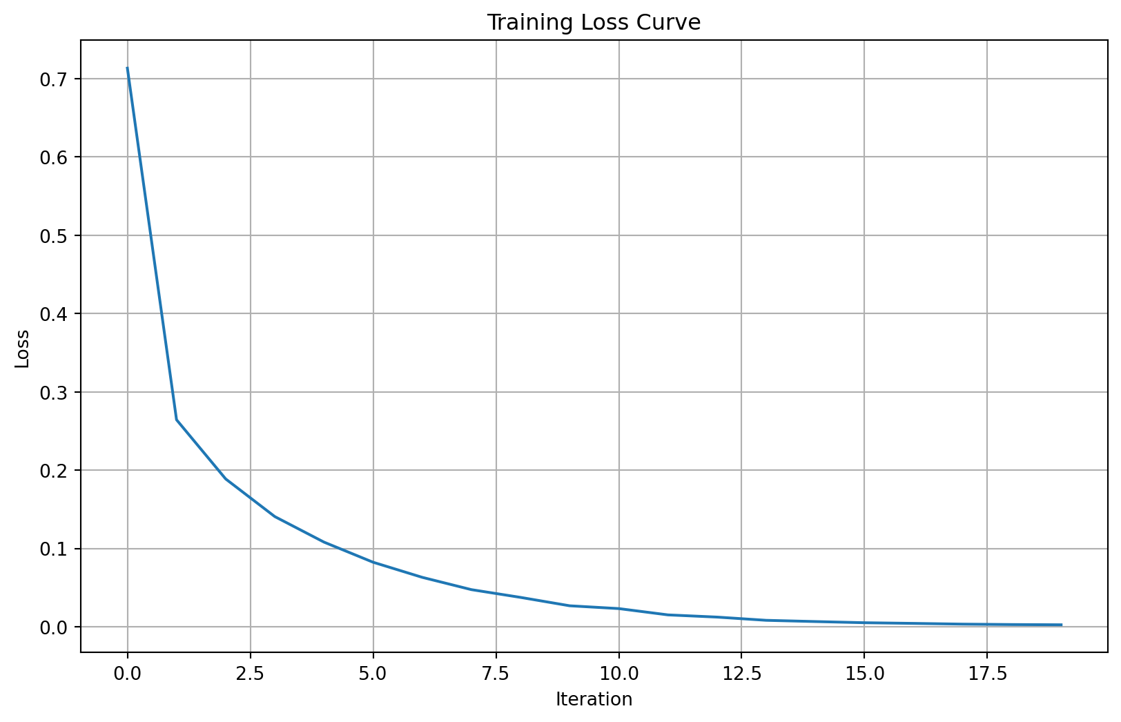
The loss curve shows how the model’s error decreases during training. A smooth decreasing curve indicates good convergence.
Let’s look at some predictions and their confidence:
# Get prediction probabilities
y_pred_proba = mlp.predict_proba(X_test_scaled)

# Visualize some predictions
fig, axes = plt.subplots(2, 5, figsize=(15, 6))
for i, ax in enumerate(axes.flat):
    ax.imshow(X_test[i].reshape(28, 28), cmap='gray')
    pred_label = y_pred[i]
    true_label = y_test[i]
    confidence = y_pred_proba[i].max()

    color = 'green' if pred_label == true_label else 'red'
    ax.set_title(f'True: {true_label}, Pred: {pred_label}\nConf: {confidence:.2f}',
                 color=color)
    ax.axis('off')
plt.tight_layout()
plt.show()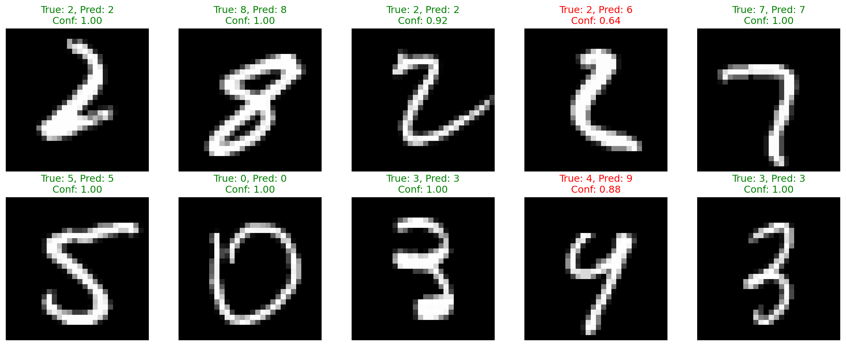
Now let’s use MLPRegressor for a regression task:
from sklearn.datasets import fetch_california_housing
from sklearn.preprocessing import StandardScaler

# Load California housing dataset
housing = fetch_california_housing()
X_housing = housing.data
y_housing = housing.target

print(f"Dataset shape: {X_housing.shape}")
print(f"Features: {housing.feature_names}")
print(f"Target: Median house value (in $100,000s)")
Dataset shape: (20640, 8)
Features: ['MedInc', 'HouseAge', 'AveRooms', 'AveBedrms', 'Population', 'AveOccup', 'Latitude', 'Longitude']
Target: Median house value (in $100,000s)# Split the data
X_train_h, X_test_h, y_train_h, y_test_h = train_test_split(
X_housing, y_housing, test_size=0.2, random_state=42
)
# Scale the features (important for neural networks!)
scaler = StandardScaler()
X_train_h_scaled = scaler.fit_transform(X_train_h)
X_test_h_scaled = scaler.transform(X_test_h)from sklearn.neural_network import MLPRegressor
mlp_reg = MLPRegressor(
hidden_layer_sizes=(100, 50),
activation='relu',
solver='adam',
alpha=0.001,
batch_size=32,
learning_rate_init=0.001,
max_iter=100,
random_state=42,
verbose=False,
early_stopping=True, # Use validation set for early stopping
validation_fraction=0.1, # 10% of training data for validation
n_iter_no_change=10 # Stop if no improvement for 10 iterations
)
print("Training MLP Regressor...")
mlp_reg.fit(X_train_h_scaled, y_train_h)
print("Training complete!")Training MLP Regressor...
Training complete!The early_stopping=True parameter automatically reserves some training data for validation and stops training when the validation score stops improving.
from sklearn.metrics import mean_squared_error, r2_score, mean_absolute_error

# Make predictions
y_pred_h = mlp_reg.predict(X_test_h_scaled)

# Calculate metrics
mse = mean_squared_error(y_test_h, y_pred_h)
rmse = np.sqrt(mse)
mae = mean_absolute_error(y_test_h, y_pred_h)
r2 = r2_score(y_test_h, y_pred_h)

print(f"Mean Squared Error: {mse:.4f}")
print(f"Root Mean Squared Error: {rmse:.4f}")
print(f"Mean Absolute Error: {mae:.4f}")
print(f"R² Score: {r2:.4f}")
Mean Squared Error: 0.2640
Root Mean Squared Error: 0.5138
Mean Absolute Error: 0.3460
R² Score: 0.7986Visualize predictions vs actual values:
fig, axes = plt.subplots(1, 2, figsize=(14, 5))

# Scatter plot
axes[0].scatter(y_test_h, y_pred_h, alpha=0.5)
axes[0].plot([y_test_h.min(), y_test_h.max()],
             [y_test_h.min(), y_test_h.max()], 'r--', lw=2)
axes[0].set_xlabel('Actual Values')
axes[0].set_ylabel('Predicted Values')
axes[0].set_title('Predicted vs Actual House Prices')
axes[0].grid(True)

# Residual plot
residuals = y_test_h - y_pred_h
axes[1].scatter(y_pred_h, residuals, alpha=0.5)
axes[1].axhline(y=0, color='r', linestyle='--', lw=2)
axes[1].set_xlabel('Predicted Values')
axes[1].set_ylabel('Residuals')
axes[1].set_title('Residual Plot')
axes[1].grid(True)

plt.tight_layout()
plt.show()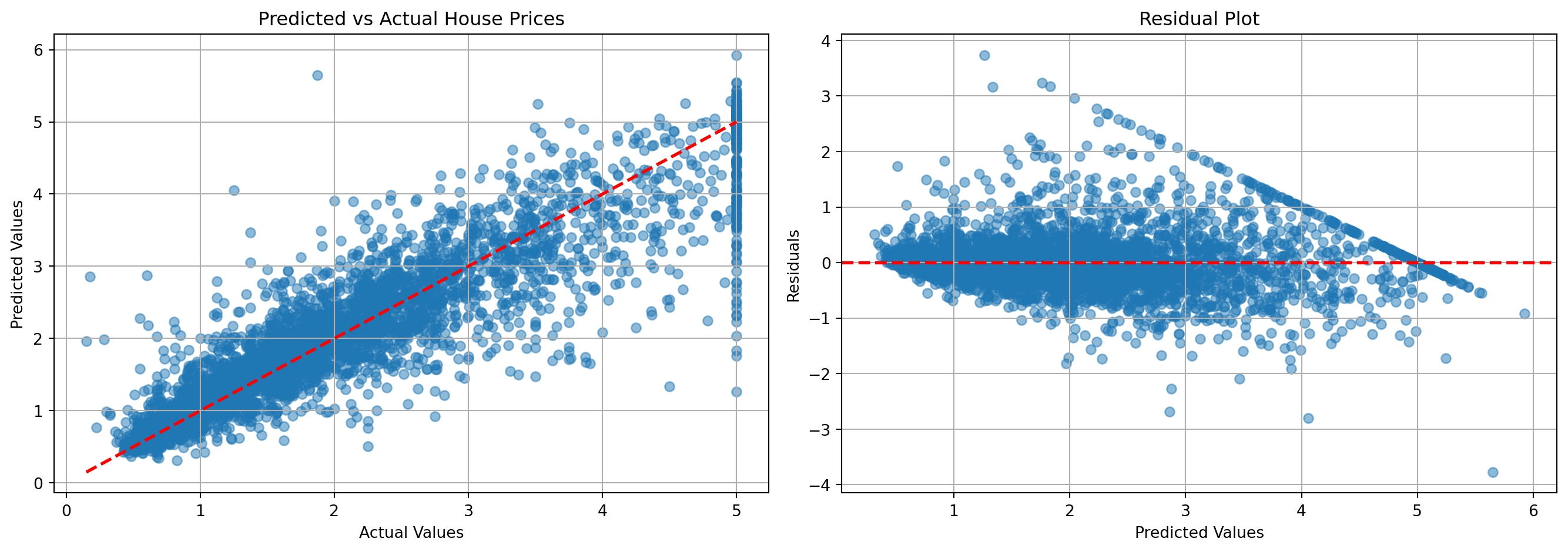
Training and validation loss curves:
plt.figure(figsize=(10, 6))
plt.plot(mlp_reg.loss_curve_, label='Training Loss')
plt.plot(mlp_reg.validation_scores_, label='Validation Score (R²)')
plt.xlabel('Iteration')
plt.ylabel('Value')
plt.title('Training Progress with Early Stopping')
plt.legend()
plt.grid(True)
plt.show()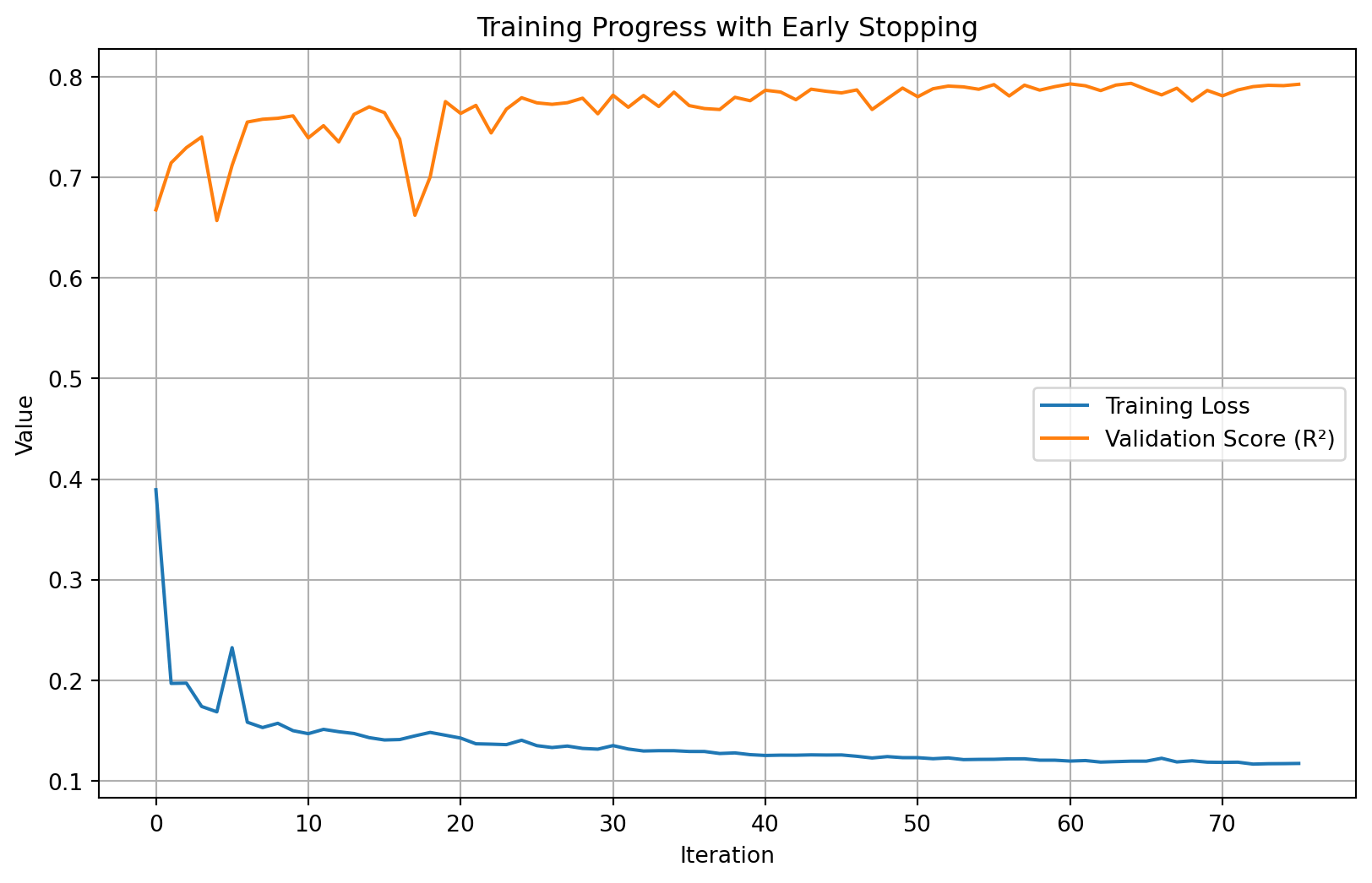
One of the advantages of scikit-learn is easy integration with hyperparameter tuning tools:
from sklearn.model_selection import GridSearchCV

# Define parameter grid (simplified for faster execution)
param_grid = {
    'hidden_layer_sizes': [(50,), (100,), (50, 50)],
    'activation': ['relu'],
    'alpha': [0.0001, 0.001]
}

# Create MLP with fewer iterations for faster grid search
mlp_grid = MLPClassifier(
    max_iter=20,
    random_state=42,
    early_stopping=True,
    validation_fraction=0.1,
    n_iter_no_change=5,
    verbose=False
)

print("Running Grid Search (this may take a while)...")
# Use a smaller subset for the grid search demo
X_grid = X_train_scaled[:1500]
y_grid = y_train[:1500]

grid_search = GridSearchCV(
    mlp_grid,
    param_grid,
    cv=3,           # 3-fold cross-validation
    n_jobs=2,       # Limit parallel jobs for better stability
    verbose=0
)

grid_search.fit(X_grid, y_grid)
print("\nBest parameters:", grid_search.best_params_)
print(f"Best cross-validation score: {grid_search.best_score_:.4f}")
Running Grid Search (this may take a while)...
Best parameters: {'activation': 'relu', 'alpha': 0.001, 'hidden_layer_sizes': (50,)}
Best cross-validation score: 0.8740
Visualize grid search results:
results_df = pd.DataFrame(grid_search.cv_results_)

# Get top configurations
n_configs = min(10, len(results_df))
top_results = results_df.nlargest(n_configs, 'mean_test_score')

plt.figure(figsize=(12, 6))
plt.barh(range(len(top_results)), top_results['mean_test_score'])
plt.yticks(range(len(top_results)),
           [f"Config {i+1}" for i in range(len(top_results))])
plt.xlabel('Mean CV Score')
plt.title('Top Hyperparameter Configurations')
plt.grid(True, axis='x')
plt.tight_layout()
plt.show()

print("\nTop configurations:")
print(top_results[['params', 'mean_test_score', 'std_test_score']].head())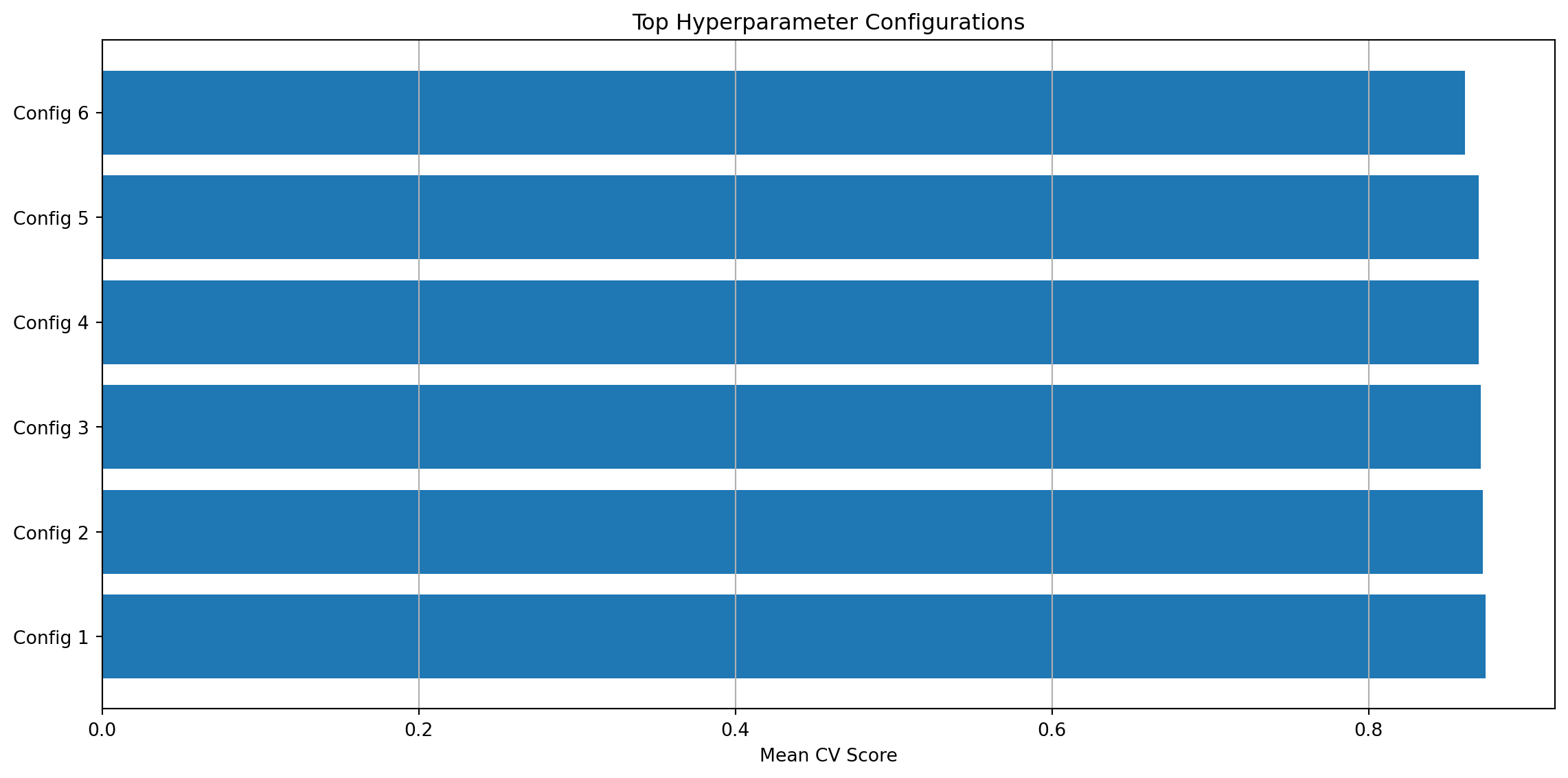
Top configurations:
                                              params  mean_test_score  \
3  {'activation': 'relu', 'alpha': 0.001, 'hidden...         0.874000
0  {'activation': 'relu', 'alpha': 0.0001, 'hidde...         0.872000
1  {'activation': 'relu', 'alpha': 0.0001, 'hidde...         0.870667
4  {'activation': 'relu', 'alpha': 0.001, 'hidden...         0.869333
5  {'activation': 'relu', 'alpha': 0.001, 'hidden...         0.869333

   std_test_score
3        0.007483
0        0.008165
1        0.016357
4        0.015861
5 0.010625 Advantages:
Best for:
Advantages:
Best for:
Let’s compare the code for creating a simple MLP:
from sklearn.neural_network import MLPClassifier

# Define and train
mlp = MLPClassifier(
    hidden_layer_sizes=(128, 64),
    activation='relu',
    max_iter=100
)
mlp.fit(X_train, y_train)

# Predict
predictions = mlp.predict(X_test)import torch
import torch.nn as nn
class MLP(nn.Module):
def __init__(self):
super().__init__()
self.layers = nn.Sequential(
nn.Linear(784, 128),
nn.ReLU(),
nn.Linear(128, 64),
nn.ReLU(),
nn.Linear(64, 10)
)
def forward(self, x):
return self.layers(x)
# Training loop required...For most standard tasks with moderate-sized datasets, scikit-learn’s MLP is perfectly adequate and much simpler to use. Save PyTorch for when you need more power and flexibility.
Scikit-learn supports adaptive learning rates:
# Adaptive learning rate
mlp_adaptive = MLPClassifier(
    hidden_layer_sizes=(100, 50),
    learning_rate='adaptive',      # Decrease learning rate when loss plateaus
    learning_rate_init=0.01,
    max_iter=50,
    random_state=42,
    verbose=False
)

mlp_adaptive.fit(X_train_scaled[:5000], y_train[:5000])
print(f"Final accuracy: {mlp_adaptive.score(X_test_scaled, y_test):.4f}")
Final accuracy: 0.9410You can continue training from where you left off:
# Initial training
mlp_warm = MLPClassifier(
    hidden_layer_sizes=(100,),
    max_iter=10,
    warm_start=True,    # Allow continued training
    random_state=42,
    verbose=False
)

print("Initial training (10 iterations)...")
mlp_warm.fit(X_train_scaled[:5000], y_train[:5000])
print(f"Accuracy after 10 iterations: {mlp_warm.score(X_test_scaled, y_test):.4f}")

# Continue training
print("\nContinued training (10 more iterations)...")
mlp_warm.set_params(max_iter=20)
mlp_warm.fit(X_train_scaled[:5000], y_train[:5000])
print(f"Accuracy after 20 iterations: {mlp_warm.score(X_test_scaled, y_test):.4f}")
Initial training (10 iterations)...
Accuracy after 10 iterations: 0.9115
Continued training (10 more iterations)...
Accuracy after 20 iterations: 0.9225For large datasets that don’t fit in memory, use partial_fit:
from sklearn.neural_network import MLPClassifier

# Create model
mlp_online = MLPClassifier(
    hidden_layer_sizes=(100,),
    random_state=42,
    warm_start=True
)

# Train in batches
batch_size = 1000
n_batches = len(X_train_scaled) // batch_size

print("Training with partial_fit...")
for i in range(min(n_batches, 5)):  # Just 5 batches for demo
    start_idx = i * batch_size
    end_idx = start_idx + batch_size

    X_batch = X_train_scaled[start_idx:end_idx]
    y_batch = y_train[start_idx:end_idx]

    # For first batch, need to specify classes
    if i == 0:
        mlp_online.partial_fit(X_batch, y_batch, classes=np.unique(y_train))
    else:
        mlp_online.partial_fit(X_batch, y_batch)

    if (i + 1) % 2 == 0:
        score = mlp_online.score(X_test_scaled, y_test)
        print(f"  Batch {i+1}/{n_batches}: Test accuracy = {score:.4f}")
Training with partial_fit...
Batch 2/8: Test accuracy = 0.6390
Batch 4/8: Test accuracy = 0.7980Always scale your features:
from sklearn.pipeline import Pipeline

# Create a pipeline with scaling and MLP
pipeline = Pipeline([
    ('scaler', StandardScaler()),
    ('mlp', MLPClassifier(hidden_layer_sizes=(100,), random_state=42))
])

# The pipeline handles scaling automatically
pipeline.fit(X_train[:1000], y_train[:1000])
accuracy = pipeline.score(X_test, y_test)
print(f"Pipeline accuracy: {accuracy:.4f}")
Pipeline accuracy: 0.8805Use cross-validation to get robust performance estimates:
from sklearn.model_selection import cross_val_score

mlp_cv = MLPClassifier(
    hidden_layer_sizes=(50,),
    max_iter=20,
    random_state=42,
    verbose=False
)

# 5-fold cross-validation
cv_scores = cross_val_score(
    mlp_cv,
    X_train_scaled[:2000],
    y_train[:2000],
    cv=5,
    n_jobs=-1
)

print(f"CV Scores: {cv_scores}")
print(f"Mean CV Score: {cv_scores.mean():.4f} (+/- {cv_scores.std() * 2:.4f})")
CV Scores: [0.8825 0.8925 0.9025 0.88 0.92 ]
Mean CV Score: 0.8955 (+/- 0.0292)Use early stopping and regularization:
# With early stopping and regularization
mlp_reg = MLPClassifier(
    hidden_layer_sizes=(100, 50),
    alpha=0.01,              # L2 regularization
    early_stopping=True,
    validation_fraction=0.2,
    n_iter_no_change=10,
    max_iter=100,
    random_state=42,
    verbose=False
)

mlp_reg.fit(X_train_scaled[:5000], y_train[:5000])
print(f"Training stopped at iteration: {mlp_reg.n_iter_}")
print(f"Best validation score: {mlp_reg.best_validation_score_:.4f}")
print(f"Test accuracy: {mlp_reg.score(X_test_scaled, y_test):.4f}")
Training stopped at iteration: 49
Best validation score: 0.9260
Test accuracy: 0.9305Different solvers work better in different scenarios:
| Solver | Best For | Notes |
|---|---|---|
'adam' |
Most cases | Good default, fast convergence |
'sgd' |
Large datasets | Need to tune learning rate carefully |
'lbfgs' |
Small datasets | Faster for small datasets, more memory |
# Example comparing solvers
solvers = ['adam', 'sgd', 'lbfgs']
results = {}

for solver in solvers:
    mlp = MLPClassifier(
        hidden_layer_sizes=(50,),
        solver=solver,
        max_iter=50,
        random_state=42,
        verbose=False
    )
    mlp.fit(X_train_scaled[:2000], y_train[:2000])
    score = mlp.score(X_test_scaled, y_test)
    results[solver] = score
    print(f"{solver:10s}: {score:.4f}")
adam : 0.9000
sgd : 0.8330
lbfgs : 0.8800If you see ConvergenceWarning, try: 1. Increase max_iter 2. Decrease learning_rate_init 3. Enable early_stopping=True 4. Check if data is properly scaled
If accuracy is low, check: 1. Is the data scaled/normalized? 2. Is the architecture appropriate for the problem? 3. Is the learning rate too high or low? 4. Do you need more training iterations? 5. Is regularization (alpha) too strong?
We covered:
MLPClassifier and MLPRegressorKey Takeaways:
Try the following on your own: