Recommender Systems – II
Introduction
In Part II, we will:
- Study a modern deep learning approach:
- Deep Learning Recommender Model (DLRM)
- Connection to Matrix Factorization
- Architecture and components
- System challenges and optimizations
- Reflect on the societal impact of recommender systems
This section draws heavily on
- Deep Learning Recommender Model for Personalization and Recommendation Systems, (Naumov et al. 2019)
Deep Learning for Recommender Systems
Why Deep Learning for Recommendations?
Modern recommender systems face unique challenges:
Scale:
- Billions of users and items
- Massive embedding tables (100s of GB to TB)
- Over 79% of AI inference cycles in production data centers (Naumov et al. 2019)
Data Types:
- Dense features: continuous (age, time, etc.)
- Sparse features: categorical (user ID, item ID)
- Need to handle both efficiently
The Economic Impact
Recommender systems drive substantial business value:
- Amazon: Up to 35% of revenue attributed to recommendations
- Netflix: 75% of movies watched come from recommendations
- Meta/Facebook: Core infrastructure for content ranking and ads
This economic importance motivates sophisticated deep learning approaches.
DLRM: Unifying Two Traditions
The Deep Learning Recommender Model (DLRM) (Naumov et al. 2019) synthesizes two historical approaches:
| Tradition | Key Concept | DLRM Component |
|---|---|---|
| RecSys/Collaborative Filtering | Latent factors, Matrix Factorization | Embeddings & Dot Products |
| Predictive Analytics | Statistical models → Deep Networks | MLPs for feature processing |
This fusion creates a model that efficiently handles both sparse and dense features.
Connection to Matrix Factorization
Recall from Part I that Matrix Factorization approximates \(R \approx WV^T\):
- User matrix \(W\) and item matrix \(V\) can be viewed as embedding tables
- The dot product \(w_i^T v_j\) predicts the rating
- DLRM generalizes this: embeddings for many categorical features, not just users/items
This is why DLRM uses dot products in the interaction layer—it’s a principled way to model feature interactions based on collaborative filtering theory.
Training and Evaluation Dataset
Criteo Ad Click-Through Rate (CTR) challenge: Kaggle Challenge, Dataset on HF
🏗️ Dataset Construction
- Each row represents a display ad served by Criteo covering 24 days
- The first column indicates whether the ad was clicked (1) or not clicked (0).
- Both positive (clicked) and negative (non-clicked) examples have been subsampled, though at different rates to keep business confidentiality.
🧱 Features
13 integer features
Mostly count-based; represent numerical properties of the ad, user, or context.26 categorical features
Values are hashed into 32-bit integers for anonymization.
The semantic meaning of these features is undisclosed.
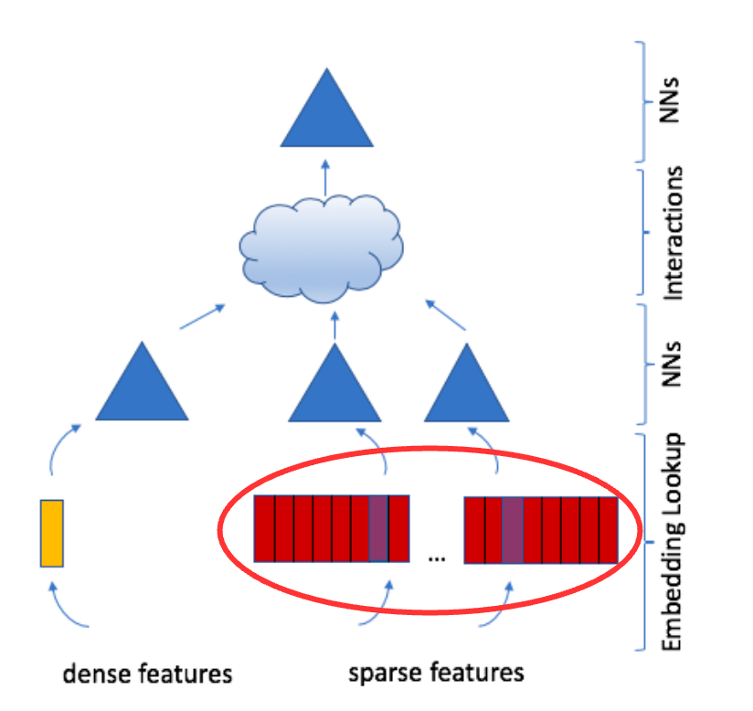
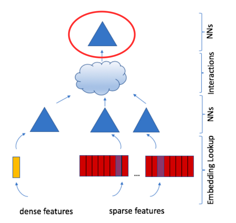
DLRM Architecture Overview
DLRM is a dual-path architecture combining sparse and dense feature processing:
Components (Figure 1):
- Embeddings: Map sparse categorical features to dense vectors
- Bottom MLP: Transform continuous features
- Feature Interaction: Explicit 2nd-order interactions via dot products
- Top MLP: Final prediction from combined features

Key Insight: Parallel processing paths that merge at the interaction layer.
Let’s examine each component to build intuition.
Embeddings
Embeddings: Map categorical inputs to latent factor space.
- A learned embedding matrix \(W \in \mathbb{R}^{m \times d}\) for each category of input
- One-hot vector \(e_i\) with \(i\text{-th}\) entry 1 and rest are 0s
- Embedding of \(e_i\) is \(i\text{-th}\) row of \(W\), i.e., \(w_i^T = e_i^T W\)
Criteo Dataset: 26 categorical features, each embedded to dimension \(d=128\).
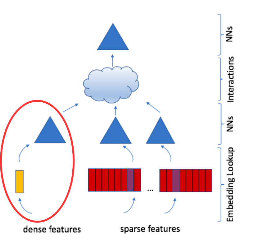
Dense Features
The advantage of the DLRM architecture is that it can take continuous features as input such as the user’s age, time of day, etc.
There is a bottom MLP that transforms these dense features into a latent space of the same dimension \(d\) as the embeddings.
Criteo Dataset Configuration:
- Input: 13 continuous (dense) features
- Bottom MLP layers: 512 → 256 → 128
- Output: 128-dimensional vector (matches embedding dimension)
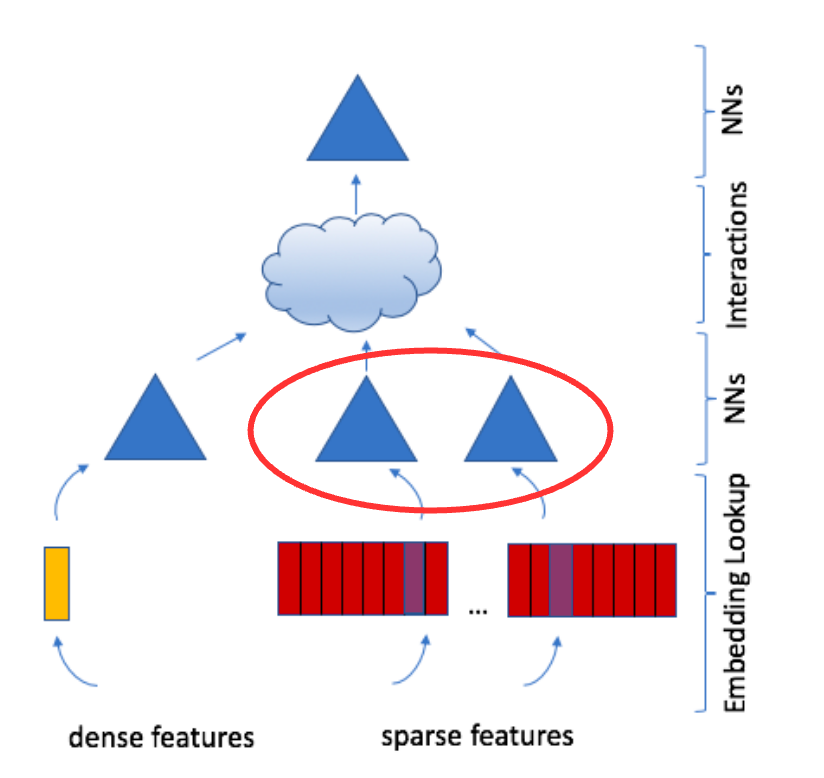
Optional Sparse Feature MLPs
Optionally, one can add MLPs to transform the sparse features as well.
Feature Interactions
Why explicit interactions?
- Simply concatenating features lets the MLP learn interactions implicitly
- But explicitly computing 2nd-order interactions is more efficient and interpretable
- Inspired by Factorization Machines from predictive analytics
How: Compute dot products of all pairs of embedding vectors and processed dense features.
Then concatenate dot products with the original dense features.
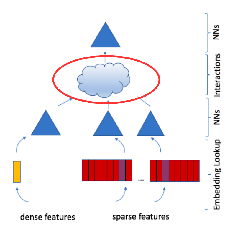
Feature Interactions, Continued
Dimensionality reduction: Using dot products between \(d\)-dimensional vectors yields scalars, avoiding the explosion of treating each element separately.
Criteo Example: 27 total vectors (1 from Bottom MLP + 26 embeddings)
- Pairwise interactions: \(\binom{27}{2} = \frac{27 \times 26}{2} = 351\) dot products
- Each dot product is a scalar (interaction strength)
Top MLP
The concatenated vector is then passed to a final MLP and then to a sigmoid function to produce the final prediction (e.g., probability score of recommendation)
This entire model is trained end-to-end using standard deep learning techniques.
Criteo Configuration:
- Input: 506-dimensional concatenated vector
- 128 processed dense features
- 351 pairwise dot products
- 27 embedding vectors (27 × 1 = 27 after pooling)
- Top MLP layers: 512 → 256 → 1
- Output: Sigmoid activation → click probability
DLRM Dimensions: Criteo Dataset Summary
Putting it all together for the Criteo Ad Kaggle dataset configuration:
| Component | Details |
|---|---|
| Input Features | 13 dense (continuous) + 26 sparse (categorical) |
| Bottom MLP | 13 → 512 → 256 → 128 |
| Embeddings | 26 categorical features × 128d each |
| Interaction Layer | 27 vectors → \(\binom{27}{2} = 351\) dot products |
| Concatenation | 128 (dense) + 351 (interactions) + 27 (pooled embeddings) = 506 |
| Top MLP | 506 → 512 → 256 → 1 |
| Output | Sigmoid(1) → Click probability |
Key observation: All vectors in interaction layer are 128-dimensional, enabling efficient pairwise dot products.
The Memory Challenge
Production-scale DLRM models face unique bottlenecks:
Memory Intensive:
- Embedding tables can be >99.9% of model memory
- Real datasets have millions of unique IDs
- Example: Criteo has 26 categorical features, some with 10M+ unique values
- Total size: 100s of GB to TB
Irregular Access Patterns:
- Embedding lookups (
SparseLengthsSum) have low compute intensity - High cache miss rates (vs. dense operations)
- Memory bandwidth becomes the bottleneck
- Different from typical DNN workloads (CNNs, RNNs)
This is why DLRM requires specialized system optimizations.
Parallelization Strategy
DLRM’s size prevents simple data parallelism (can’t replicate massive embedding tables).
Solution: Hybrid Model + Data Parallelism
Model Parallelism for embeddings:
- Distribute embedding tables across devices
- Each device stores subset of embeddings
- Reduces memory per device
Data Parallelism for MLPs:
- MLPs have fewer parameters
- Can replicate across devices
- Process different samples in parallel
Communication: Use “butterfly shuffle” (personalized all-to-all) to gather embeddings for the interaction layer.
Training Results
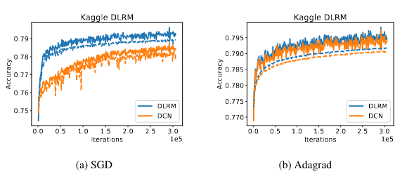
Figure 2 shows the training (solid) and validation (dashed) accuracies of DLRM on the Criteo Ad Kaggle dataset.
DLRM achieves comparable or better accuracy than Deep and Cross Network (DCN) (Wang et al. 2017), while being more efficient for sparse feature interactions.
Other Modern Approaches
There are many other modern approaches to recommender systems for example:
- Graph-Based Recommender Systems:
- Leverage graph structures to capture relationships between users and items.
- Use techniques like Graph Neural Networks (GNNs) to enhance recommendation accuracy.
- Context-Aware Recommender Systems:
- Incorporate contextual information such as time, location, and user mood to provide more personalized recommendations.
- Contextual data can be integrated using various machine learning models.
- Hybrid Recommender Systems:
- Combine multiple recommendation techniques, such as collaborative filtering and content-based filtering, to improve performance.
- Aim to leverage the strengths of different methods while mitigating their weaknesses.
- Reinforcement Learning-Based Recommender Systems:
- Use reinforcement learning to optimize long-term user engagement and satisfaction.
- Models learn to make sequential recommendations by interacting with users and receiving feedback.
These approaches often leverage advancements in machine learning and data processing to provide more accurate and personalized recommendations.
See (Ricci et al. 2022) for a comprehensive overview of recommender systems.
Impact of Recommender Systems
Filter Bubbles
There are a number of concerns with the widespread use of recommender systems and personalization in society.
First, recommender systems are accused of creating filter bubbles.
A filter bubble is the tendency for recommender systems to limit the variety of information presented to the user.
The concern is that a user’s past expression of interests will guide the algorithm in continuing to provide “more of the same.”
This is believed to increase polarization in society, and to reinforce confirmation bias.
Maximizing Engagement
Second, recommender systems in modern usage are often tuned to maximize engagement.
In other words, the objective function of the system is not to present the user’s most favored content, but rather the content that will be most likely to keep the user on the site.
How this works in practice:
- Objective Functions: Models optimize for metrics like click-through rate, watch time, or session duration
- A/B Testing: Continuous experimentation to find which content keeps users engaged longer
- Feedback Loops: User interactions train the model to predict and serve “sticky” content
The Incentive: Sites supported by advertising revenue directly benefit from more engagement time. More engagement means more ad impressions and more revenue.
Extreme Content
However, many studies have shown that sites that strive to maximize engagement do so in large part by guiding users toward extreme content:
- content that is shocking,
- or feeds conspiracy theories,
- or presents extreme views on popular topics.
Given this tendency of modern recommender systems, for a third party to create “clickbait” content such as this, one of the easiest ways is to present false claims.
Methods for addressing these issues are being very actively studied at present.
Ways of addressing these issues can be:
- via technology
- via public policy
Recap and References
BU CS/CDS Research
You can read about some of the work done in Professor Mark Crovella’s group on this topic:
- How YouTube Leads Privacy-Seeking Users Away from Reliable Information, (Spinelli and Crovella 2020)
- Closed-Loop Opinion Formation, (Spinelli and Crovella 2017)
- Fighting Fire with Fire: Using Antidote Data to Improve Polarization and Fairness of Recommender Systems, (Rastegarpanah et al. 2019)
Recap
Part I (Collaborative Filtering & Matrix Factorization):
- Collaborative filtering (CF): user-user and item-item similarity approaches
- Matrix factorization (MF): latent vectors and ALS optimization
- Practical implementation of ALS on Amazon movie reviews
Part II (Deep Learning & Impact):
- DLRM: A production-scale deep learning approach unifying RecSys and predictive analytics traditions
- Connection between embeddings and matrix factorization latent factors
- DLRM architecture: dual-path design with explicit feature interactions
- System challenges: massive embedding tables (>99.9% of model memory) and irregular memory access
- Parallelization: hybrid model + data parallelism with butterfly shuffle communication
- Societal impact: filter bubbles, engagement maximization, and extreme content concerns