Essential Tools: Pandas

Introduction

In this lecture we discuss one of most useful Python packages for data science – Pandas.

We’ll touch on some highlights here, but to learn more, start with the Pandas Getting started tutorials

Pandas

Pandas is a Python library for data manipulation and analysis with an emphasis on tabular data.
It can be used to produce high quality plots and integrates nicely with other libraries that expect NumPy arrays.
Knowledge and use of Pandas is essential as a data scientist.

The most important data structure provided by Pandas is the DataFrame implemented in the DataFrame class.

Unlike a numpy array, a DataFrame can have columns of different types.

Make it a habit that when you’re given a tabular dataset, load it into a DataFrame.

Fetching, storing and retrieving your data

We’ll work with stock data. A popular python package for this is yfinance, but there seems to be some access rate limits which make it more difficult to use.

Instead we’ll manually download a CSV file:

MANUAL DOWNLOAD FROM WALL STREET JOURNAL:

1. Go to: https://www.wsj.com/market-data/quotes/NVDA/historical-prices
2. Set date range: January 1, 2024 to December 31, 2024
3. Click "Download" button
4. Save the CSV file
5. Load in Python:

import pandas as pd

try:
    nvidia_stocks = pd.read_csv('data/stocks/nvidia_stock_2024.csv', index_col=0)
except FileNotFoundError:
    url = 'https://raw.githubusercontent.com/tools4ds/DS701-Course-Notes/main/ds701_book/data/stocks/nvidia_stock_2024.csv'
    nvidia_stocks = pd.read_csv(url, index_col=0)

nvidia_stocks = nvidia_stocks.sort_index()

It’s important to inspect the data you are working with and Pandas provides a variety of methods to do so such as .head(), .tail(), .info(), .describe(), etc.

nvidia_stocks.head()

	Open	High	Low	Close	Volume
Date
01/02/24	49.244	49.2950	47.595	48.168	4.112542e+08
01/03/24	47.485	48.1841	47.320	47.569	3.208962e+08
01/04/24	47.767	48.5000	47.508	47.998	3.065349e+08
01/05/24	48.462	49.5470	48.306	49.097	4.150393e+08
01/08/24	49.512	52.2750	49.479	52.253	6.425099e+08

Notice how each row has a label and each column has a label.

A DataFrame is a python object that has many associated methods to explore and manipulate the data.

The method .info() gives you a description of the dataframe.

nvidia_stocks.info()

<class 'pandas.core.frame.DataFrame'>
Index: 252 entries, 01/02/24 to 12/31/24
Data columns (total 5 columns):
 #   Column  Non-Null Count  Dtype  
---  ------  --------------  -----  
 0   Open    252 non-null    float64
 1   High    252 non-null    float64
 2   Low     252 non-null    float64
 3   Close   252 non-null    float64
 4   Volume  252 non-null    float64
dtypes: float64(5)
memory usage: 11.8+ KB

The method .describe() gives you summary statistics of the dataframe.

nvidia_stocks.describe()

	Open	High	Low	Close	Volume
count	252.000000	252.000000	252.000000	252.000000	2.520000e+02
mean	107.899121	109.852719	105.631198	107.825438	3.773571e+08
std	27.145281	27.437677	26.575767	26.957320	1.618595e+08
min	47.485000	48.184100	47.320000	47.569000	1.051570e+08
25%	87.740500	89.479750	86.128550	87.751500	2.498443e+08
50%	115.950000	117.090000	111.791500	115.295000	3.508633e+08
75%	130.282500	133.542500	128.235000	130.462500	4.752442e+08
max	149.350000	152.890000	146.260000	148.880000	1.142269e+09

Writing/Reading to/from a `.csv` file

Pandas can read and write dataframes with many file formats such as .csv, .json, .parquet, .xlsx, .html, SQL, etc.

Here we write the dataframe to a .csv file.

nvidia_stocks.to_csv('nvidia_data.csv')

We can escape a shell command using the ! operator to see the top of the file.

!head nvidia_data.csv

Date,Open,High,Low,Close,Volume
01/02/24,49.244,49.295,47.595,48.168,411254215.887458
01/03/24,47.485,48.1841,47.32,47.569,320896186.791038
01/04/24,47.767,48.5,47.508,47.998,306534876.934651
01/05/24,48.462,49.547,48.306,49.097,415039295.849607
01/08/24,49.512,52.275,49.479,52.253,642509873.574901
01/09/24,52.401,54.325,51.69,53.14,773100072.268999
01/10/24,53.616,54.6,53.489,54.35,533795774.662042
01/11/24,54.999,55.346,53.56,54.822,596758784.032412
01/12/24,54.62,54.97,54.3301,54.71,352993586.470064

And of course we can likewise read a .csv file into a dataframe. This is probably the most common way you will get data into Pandas.

df = pd.read_csv('nvidia_data.csv')
df.head()

	Date	Open	High	Low	Close	Volume
0	01/02/24	49.244	49.2950	47.595	48.168	4.112542e+08
1	01/03/24	47.485	48.1841	47.320	47.569	3.208962e+08
2	01/04/24	47.767	48.5000	47.508	47.998	3.065349e+08
3	01/05/24	48.462	49.5470	48.306	49.097	4.150393e+08
4	01/08/24	49.512	52.2750	49.479	52.253	6.425099e+08

Caution

But be careful, the index column is not automatically set.

df.info()

<class 'pandas.core.frame.DataFrame'>
RangeIndex: 252 entries, 0 to 251
Data columns (total 6 columns):
 #   Column  Non-Null Count  Dtype  
---  ------  --------------  -----  
 0   Date    252 non-null    object 
 1   Open    252 non-null    float64
 2   High    252 non-null    float64
 3   Low     252 non-null    float64
 4   Close   252 non-null    float64
 5   Volume  252 non-null    float64
dtypes: float64(5), object(1)
memory usage: 11.9+ KB

Note the index description.

To set the index column, we can use the index_col parameter.

df = pd.read_csv('nvidia_data.csv', index_col=0)
df.info()

<class 'pandas.core.frame.DataFrame'>
Index: 252 entries, 01/02/24 to 12/31/24
Data columns (total 5 columns):
 #   Column  Non-Null Count  Dtype  
---  ------  --------------  -----  
 0   Open    252 non-null    float64
 1   High    252 non-null    float64
 2   Low     252 non-null    float64
 3   Close   252 non-null    float64
 4   Volume  252 non-null    float64
dtypes: float64(5)
memory usage: 11.8+ KB

Working with data columns

In general, we’ll typically describe the rows in the dataframe as items (or observations or data samples) and the columns as features.

df.columns

Index(['Open', 'High', 'Low', 'Close', 'Volume'], dtype='object')

Pandas allows you to reference a column similar to a python dictionary key, using column names in square brackets.

df['Open']

Date
01/02/24     49.244
01/03/24     47.485
01/04/24     47.767
01/05/24     48.462
01/08/24     49.512
             ...   
12/24/24    140.000
12/26/24    139.700
12/27/24    138.550
12/30/24    134.830
12/31/24    138.030
Name: Open, Length: 252, dtype: float64

Note that this returns a Series object, the other fundamental data structure in Pandas.

type(df['Open'])

pandas.core.series.Series

Also note that Series is indexed in this case by dates rather than simple integers.

Pandas also allows you to refer to columns using an object attribute syntax.

Note that the column name cannot include a space in this case.

df.Open

Date
01/02/24     49.244
01/03/24     47.485
01/04/24     47.767
01/05/24     48.462
01/08/24     49.512
             ...   
12/24/24    140.000
12/26/24    139.700
12/27/24    138.550
12/30/24    134.830
12/31/24    138.030
Name: Open, Length: 252, dtype: float64

You can select a list of columns:

df[['Open', 'Close']].head()

	Open	Close
Date
01/02/24	49.244	48.168
01/03/24	47.485	47.569
01/04/24	47.767	47.998
01/05/24	48.462	49.097
01/08/24	49.512	52.253

Which is just another dataframe, which is why we can chain the .head() method.

type(df[['Open', 'Close']])

pandas.core.frame.DataFrame

Changing column names is as simple as assigning to the .columns property.

Let’s adjust the column names to remove spaces.

new_column_names = [x.lower().replace(' ', '_') for x in df.columns]
df.columns = new_column_names
df.info()

<class 'pandas.core.frame.DataFrame'>
Index: 252 entries, 01/02/24 to 12/31/24
Data columns (total 5 columns):
 #   Column  Non-Null Count  Dtype  
---  ------  --------------  -----  
 0   open    252 non-null    float64
 1   high    252 non-null    float64
 2   low     252 non-null    float64
 3   close   252 non-null    float64
 4   volume  252 non-null    float64
dtypes: float64(5)
memory usage: 19.9+ KB

Observe that we first created a list of column names without spaces using list comprehension. This is the pythonic way to generate a new list.

Now all columns can be accessed using the dot notation.

A sampling of DataFrame methods.

There are many useful methods in the DataFrame object. It is important to familiarize yourself with these methods.

The following methods calculate the mean, standard deviation, and median of the specified numeric columns.

df.mean()

open      1.078991e+02
high      1.098527e+02
low       1.056312e+02
close     1.078254e+02
volume    3.773571e+08
dtype: float64

or we can give a list of columns to the Dataframe object:

df[['open', 'close', 'volume']].mean()

open      1.078991e+02
close     1.078254e+02
volume    3.773571e+08
dtype: float64

df.std()

open      2.714528e+01
high      2.743768e+01
low       2.657577e+01
close     2.695732e+01
volume    1.618595e+08
dtype: float64

df.median()

open      1.159500e+02
high      1.170900e+02
low       1.117915e+02
close     1.152950e+02
volume    3.508633e+08
dtype: float64

Or apply the method to a single column:

df.open.mean()

np.float64(107.89912063492064)

df.high.mean()

np.float64(109.85271904761905)

Plotting methods

Pandas also wraps matplotlib and provides a variety of easy-to-use plotting functions directly from the dataframe object.

These are your “first look” functions and useful in exploratory data analysis.

Later, we will use more specialized graphics packages to create more sophisticated visualizations.

import matplotlib.pyplot as plt

df.high.plot(label='High')
df.low.plot(label='Low')
plt.title('NVIDIA Stock Price')
plt.ylabel('Dollars')
plt.legend(loc='best')
plt.show()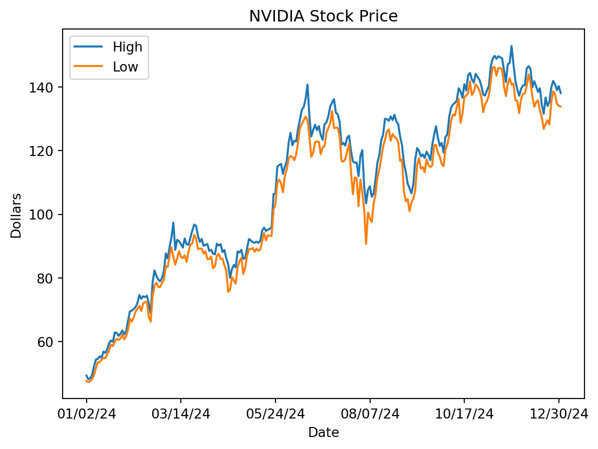

Or a histogram on the adjusted closing price.

df.close.hist()
plt.xlabel('Closing Price')
plt.ylabel('Dollars')
plt.title('NVIDIA Stock Price')
plt.show()

Accessing rows of the DataFrame

So far we’ve seen how to access a column of the DataFrame. To access a row we use different syntax.

To access a row by its index label, use the .loc() method (‘location’).

df.loc['01/02/24']

open      4.924400e+01
high      4.929500e+01
low       4.759500e+01
close     4.816800e+01
volume    4.112542e+08
Name: 01/02/24, dtype: float64

As a tangent, we can use the .apply() method to format the output.

df.loc['01/02/24'].apply(lambda x: '{:,.2f}'.format(x) if isinstance(x, (int, float)) else x)

open               49.24
high               49.30
low                47.59
close              48.17
volume    411,254,215.89
Name: 01/02/24, dtype: object

To access a row by its index number (i.e., like an array index), use .iloc() (‘integer location’)

df.iloc[0, :]

open      4.924400e+01
high      4.929500e+01
low       4.759500e+01
close     4.816800e+01
volume    4.112542e+08
Name: 01/02/24, dtype: float64

and similarly formatted:

df.iloc[0, :].apply(lambda x: '{:,.2f}'.format(x) if isinstance(x, (int, float)) else x)

open               49.24
high               49.30
low                47.59
close              48.17
volume    411,254,215.89
Name: 01/02/24, dtype: object

To iterate over the rows you can use .iterrows().

num_positive_days = 0
for idx, row in df.iterrows():
    if row.close > row.open:
        num_positive_days += 1

print(f"The total number of positive-gain days is {num_positive_days} out of {len(df)} days or as percentage {num_positive_days/len(df):.2%}")

The total number of positive-gain days is 134 out of 252 days or as percentage 53.17%

Note

This is only capturing the intraday gain/loss, not the cumulative inter-day gain/loss.

Filtering

It is easy to select rows from the data.

All the operations below return a new Series or DataFrame, which itself can be treated the same way as all Series and DataFrames we have seen so far.

tmp_high = df.high > 100
tmp_high.tail()

Date
12/24/24    True
12/26/24    True
12/27/24    True
12/30/24    True
12/31/24    True
Name: high, dtype: bool

Summing a Boolean array is the same as counting the number of True values.

sum(tmp_high)

Now, let’s select only the rows of df that correspond to tmp_high.

Note

We can pass a series to the dataframe to select rows.

df[tmp_high]

	open	high	low	close	volume
Date
05/23/24	102.028	106.3200	101.520	103.799	8.350653e+08
05/24/24	104.449	106.4750	103.000	106.469	4.294937e+08
05/28/24	110.244	114.9390	109.883	113.901	6.527280e+08
05/29/24	113.050	115.4920	110.901	114.825	5.574419e+08
05/30/24	114.650	115.8192	109.663	110.500	4.873503e+08
...	...	...	...	...	...
12/24/24	140.000	141.9000	138.650	140.220	1.051570e+08
12/26/24	139.700	140.8500	137.730	139.930	1.165191e+08
12/27/24	138.550	139.0200	134.710	137.010	1.705826e+08
12/30/24	134.830	140.2700	134.020	137.490	1.677347e+08
12/31/24	138.030	138.0700	133.830	134.290	1.556592e+08

153 rows × 5 columns

Putting it all together, we can count the number of positive days without iterating over the rows.

positive_days = df[df.close > df.open]
print(f"Total number of positive-gain days is {len(positive_days)}")
positive_days.head()

Total number of positive-gain days is 134

	open	high	low	close	volume
Date
01/03/24	47.485	48.1841	47.320	47.569	3.208962e+08
01/04/24	47.767	48.5000	47.508	47.998	3.065349e+08
01/05/24	48.462	49.5470	48.306	49.097	4.150393e+08
01/08/24	49.512	52.2750	49.479	52.253	6.425099e+08
01/09/24	52.401	54.3250	51.690	53.140	7.731001e+08

Or count the number of days with a gain of more than $2.

very_positive_days = df[(df.close - df.open) > 2]
print(f"Total number of days with gain > $2 is {len(very_positive_days)}")
very_positive_days.head()

Total number of days with gain > $2 is 51

	open	high	low	close	volume
Date
01/08/24	49.512	52.275	49.479	52.253	6.425099e+08
02/02/24	63.974	66.600	63.690	66.160	4.765777e+08
02/22/24	75.025	78.575	74.220	78.538	8.650997e+08
03/01/24	80.000	82.300	79.435	82.279	4.791351e+08
03/07/24	90.158	92.767	89.602	92.669	6.081191e+08

Note that this doesn’t the explain the total gain for the year. Why?

Creating new columns

To create a new column, simply assign values to it. The column name is similar to a key in a dictionary.

Let’s look at the daily change in closing price.

# Calculate the daily change in closing price
df['daily_change'] = df['close'].diff()

# Create the cumulative profit column
df['cum_profit'] = df['daily_change'].cumsum()

# Display the first few rows to verify the new column
print(df[['close', 'daily_change', 'cum_profit']].head())

           close  daily_change  cum_profit
Date                                      
01/02/24  48.168           NaN         NaN
01/03/24  47.569        -0.599      -0.599
01/04/24  47.998         0.429      -0.170
01/05/24  49.097         1.099       0.929
01/08/24  52.253         3.156       4.085

It is convenient that .diff() by default is the difference between the current and previous row.

Let’s look at the histogram of the daily change in stock price.

# Plot histogram of daily_change
plt.figure(figsize=(10, 6))
df['daily_change'].hist(bins=50, edgecolor='black')
plt.title('Histogram of Daily Change in Stock Price')
plt.xlabel('Daily Change')
plt.ylabel('Frequency')
plt.show()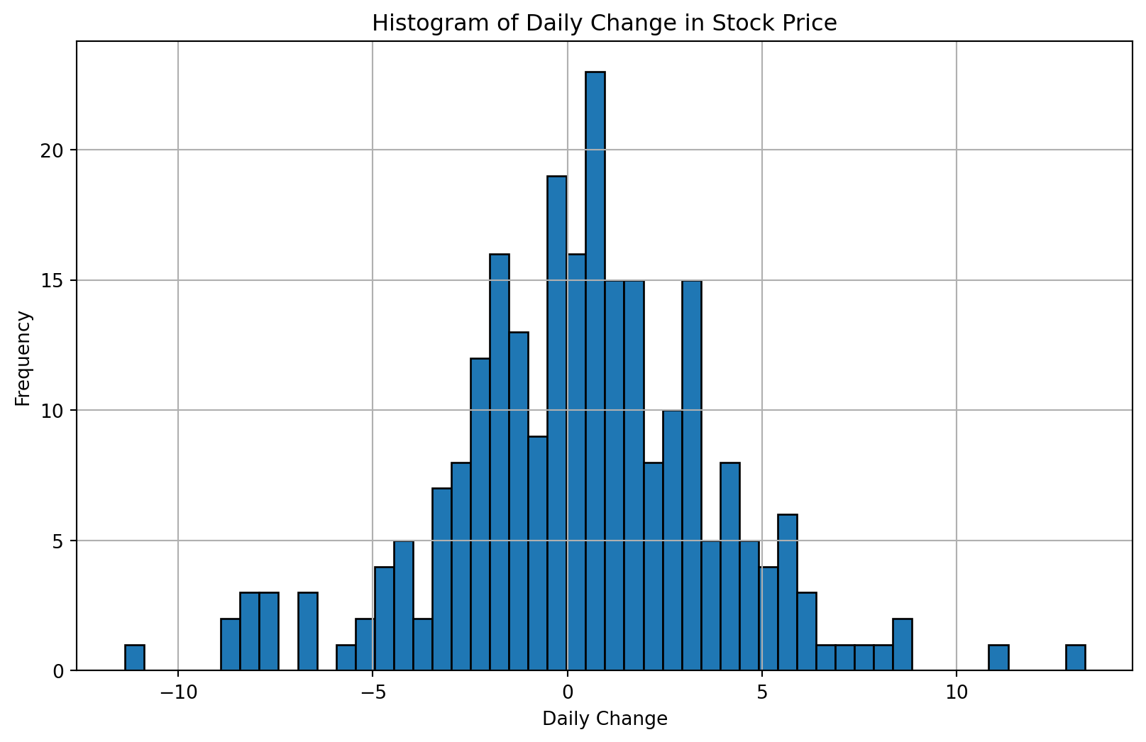

Let’s give each row a gain value as a categorical variable.

for idx, row in df.iterrows():
    if row.daily_change < 0:
        df.loc[idx,'cat_gain']='negative'
    elif row.daily_change < 1:
        df.loc[idx,'cat_gain']='small_gain'
    elif row.daily_change < 2:
        df.loc[idx,'cat_gain']='medium_gain'
    elif row.daily_change >= 2:
        df.loc[idx,'cat_gain']='large_gain'
df.head()

	open	high	low	close	volume	daily_change	cum_profit	cat_gain
Date
01/02/24	49.244	49.2950	47.595	48.168	4.112542e+08	NaN	NaN	NaN
01/03/24	47.485	48.1841	47.320	47.569	3.208962e+08	-0.599	-0.599	negative
01/04/24	47.767	48.5000	47.508	47.998	3.065349e+08	0.429	-0.170	small_gain
01/05/24	48.462	49.5470	48.306	49.097	4.150393e+08	1.099	0.929	medium_gain
01/08/24	49.512	52.2750	49.479	52.253	6.425099e+08	3.156	4.085	large_gain

Here is another, more “functional”, way to accomplish the same thing.

First, let’s drop the gain column so we can start fresh.

df.drop('cat_gain', axis=1, inplace=True)
df.head()

	open	high	low	close	volume	daily_change	cum_profit
Date
01/02/24	49.244	49.2950	47.595	48.168	4.112542e+08	NaN	NaN
01/03/24	47.485	48.1841	47.320	47.569	3.208962e+08	-0.599	-0.599
01/04/24	47.767	48.5000	47.508	47.998	3.065349e+08	0.429	-0.170
01/05/24	48.462	49.5470	48.306	49.097	4.150393e+08	1.099	0.929
01/08/24	49.512	52.2750	49.479	52.253	6.425099e+08	3.156	4.085

Define a function that classifies rows, and apply it to each row.

def namerow(row):
    if row.daily_change < 0:
        return 'negative'
    elif row.daily_change < 1:
        return 'small_gain'
    elif row.daily_change < 2:
        return 'medium_gain'
    elif row.daily_change >= 2:
        return 'large_gain'

df['cat_gain'] = df.apply(namerow, axis=1)
df.head()

	open	high	low	close	volume	daily_change	cum_profit	cat_gain
Date
01/02/24	49.244	49.2950	47.595	48.168	4.112542e+08	NaN	NaN	None
01/03/24	47.485	48.1841	47.320	47.569	3.208962e+08	-0.599	-0.599	negative
01/04/24	47.767	48.5000	47.508	47.998	3.065349e+08	0.429	-0.170	small_gain
01/05/24	48.462	49.5470	48.306	49.097	4.150393e+08	1.099	0.929	medium_gain
01/08/24	49.512	52.2750	49.479	52.253	6.425099e+08	3.156	4.085	large_gain

Understanding pandas DataFrame.groupby()

Introduction

The groupby() function is one of the most powerful tools in pandas for data analysis. It implements the “split-apply-combine” pattern:

Split your data into groups based on some criteria
Apply a function to each group independently
Combine the results back into a data structure

Think of it like organizing a deck of cards by suit, then counting how many cards are in each suit, then presenting those counts in a summary table.

Basic Concept

Imagine you have a dataset of student grades:

import pandas as pd

data = {
    'student': ['Alice', 'Bob', 'Alice', 'Bob', 'Charlie', 'Charlie'],
    'subject': ['Math', 'Math', 'English', 'English', 'Math', 'English'],
    'score': [85, 78, 92, 88, 95, 90]
}

df = pd.DataFrame(data)
print(df)

   student  subject  score
0    Alice     Math     85
1      Bob     Math     78
2    Alice  English     92
3      Bob  English     88
4  Charlie     Math     95
5  Charlie  English     90

Example 1: Simple Grouping

Let’s find the average score for each student:

# Group by student and calculate mean
result = df.groupby('student')['score'].mean()
print(result)

student
Alice      88.5
Bob        83.0
Charlie    92.5
Name: score, dtype: float64

What happened?

pandas split the data into 3 groups (one per student)
Applied the mean() function to each group’s scores
Combined the results into a Series indexed by the student names

Example 2: Multiple Aggregations

You can apply multiple functions at once:

# Multiple aggregations
result = df.groupby('student')['score'].agg(['mean', 'min', 'max', 'count'])
print(result)

         mean  min  max  count
student                       
Alice    88.5   85   92      2
Bob      83.0   78   88      2
Charlie  92.5   90   95      2

where the list in the agg() method is both a list of functions to apply to the column and a list of names for the columns in the resulting DataFrame.

What happened?

pandas split the data into 3 groups (one per student)
Applied the mean(), min(), max(), and count() functions to each group’s scores
Combined the results into a DataFrame indexed by the student names with the column names being the functions applied to the scores.

Example 3: Grouping by Multiple Columns

What if we want to see scores grouped by both student AND subject?

# Group by multiple columns
result = df.groupby(['student', 'subject'])['score'].mean()
print(result)

student  subject
Alice    English    92.0
         Math       85.0
Bob      English    88.0
         Math       78.0
Charlie  English    90.0
         Math       95.0
Name: score, dtype: float64

This creates a hierarchical index (MultiIndex) with two levels.

Example 4: Aggregating Multiple Columns

Let’s add more data:

data = {
    'student': ['Alice', 'Bob', 'Alice', 'Bob', 'Charlie', 'Charlie'],
    'subject': ['Math', 'Math', 'English', 'English', 'Math', 'English'],
    'score': [85, 78, 92, 88, 95, 90],
    'hours_studied': [5, 3, 6, 4, 7, 5]
}

df = pd.DataFrame(data)

# Group by student and get mean of all numeric columns
result = df.groupby('student')[['score', 'hours_studied']].mean()
print(result)

         score  hours_studied
student                      
Alice     88.5            5.5
Bob       83.0            3.5
Charlie   92.5            6.0

Example 5: Different Aggregations for Different Columns

You can apply different functions to different columns:

# Different aggregations for different columns
result = df.groupby('student').agg({
    'score': ['mean', 'max'],
    'hours_studied': 'sum'
})
print(result)

        score     hours_studied
         mean max           sum
student                        
Alice    88.5  92            11
Bob      83.0  88             7
Charlie  92.5  95            12

Example 6: Using Custom Functions

You can define your own aggregation functions:

# Custom function: range (max - min)
def score_range(x):
    return x.max() - x.min()

result = df.groupby('student')['score'].agg([
    'mean',
    ('range', score_range)
])
print(result)

         mean  range
student             
Alice    88.5      7
Bob      83.0     10
Charlie  92.5      5

where the argument ('range', score_range) is a tuple with the name of the column in the resulting DataFrame and the function to apply to the column.

What happened?

pandas split the data into 3 groups (one per student)
Applied the mean() function to the scores column
Applied the score_range() function to the scores column and named the column range in the resulting DataFrame
Combined the results into a DataFrame indexed by the student names with the column names being the functions applied to the scores.

Example 7: Filtering Groups

You can filter out entire groups based on conditions:

# Only keep students with average score above 85
result = df.groupby('student').filter(lambda x: x['score'].mean() > 85)
print(result)

   student  subject  score  hours_studied
0    Alice     Math     85              5
2    Alice  English     92              6
4  Charlie     Math     95              7
5  Charlie  English     90              5

Example 8: Transform - Keeping Original Shape

Sometimes you want to add group statistics to your original dataframe:

# Add a column with each student's average score
df['student_avg'] = df.groupby('student')['score'].transform('mean')
print(df)

   student  subject  score  hours_studied  student_avg
0    Alice     Math     85              5         88.5
1      Bob     Math     78              3         83.0
2    Alice  English     92              6         88.5
3      Bob  English     88              4         83.0
4  Charlie     Math     95              7         92.5
5  Charlie  English     90              5         92.5

Notice how transform() returns a Series with the same length as the original DataFrame, broadcasting the group statistic to all rows in that group.

Example 9: Apply - Maximum Flexibility

The apply() method gives you complete control and can return different shapes:

# Use apply() to get multiple statistics per group
def analyze_student(group):
    return pd.Series({
        'avg_score': group['score'].mean(),
        'score_range': group['score'].max() - group['score'].min(),
        'total_hours': group['hours_studied'].sum(),
        'efficiency': group['score'].mean() / group['hours_studied'].mean()
    })

result = df.groupby('student').apply(analyze_student, include_groups=False)
print(result)

         avg_score  score_range  total_hours  efficiency
student                                                 
Alice         88.5          7.0         11.0   16.090909
Bob           83.0         10.0          7.0   23.714286
Charlie       92.5          5.0         12.0   15.416667

Note: Unlike transform() which must return the same shape as the input, apply() can return aggregated results of any shape.

Example 10: Iterating Over Groups

Sometimes you need to process each group separately:

# Iterate over groups
for name, group in df.groupby('student'):
    print(f"\n{name}'s records:")
    print(group)


Alice's records:
  student  subject  score  hours_studied  student_avg
0   Alice     Math     85              5         88.5
2   Alice  English     92              6         88.5

Bob's records:
  student  subject  score  hours_studied  student_avg
1     Bob     Math     78              3         83.0
3     Bob  English     88              4         83.0

Charlie's records:
   student  subject  score  hours_studied  student_avg
4  Charlie     Math     95              7         92.5
5  Charlie  English     90              5         92.5

Common Aggregation Functions

Here are the most commonly used aggregation functions:

count() - Number of non-null values
sum() - Sum of values
mean() - Average of values
median() - Median value
min() - Minimum value
max() - Maximum value
std() - Standard deviation
var() - Variance
first() - First value in group
last() - Last value in group
size() - Number of rows (including NaN)

Example 11: (Synthetic) Sales Data Analysis

# Sample sales data
sales_data = {
    'date': pd.date_range('2024-01-01', periods=12, freq='ME'),
    'region': ['North', 'South', 'North', 'South', 'North', 'South',
               'North', 'South', 'North', 'South', 'North', 'South'],
    'product': ['A', 'A', 'B', 'B', 'A', 'A', 'B', 'B', 'A', 'A', 'B', 'B'],
    'sales': [100, 150, 200, 175, 110, 165, 210, 180, 120, 170, 220, 190],
    'units': [10, 15, 20, 17, 11, 16, 21, 18, 12, 17, 22, 19]
}

sales_df = pd.DataFrame(sales_data)
print(sales_df)

# Comprehensive analysis by region
analysis = sales_df.groupby('region').agg({
    'sales': ['sum', 'mean', 'max'],
    'units': 'sum',
    'product': 'count'  # Count of transactions
})

print("\nAnalysis:")
print(analysis)

         date region product  sales  units
0  2024-01-31  North       A    100     10
1  2024-02-29  South       A    150     15
2  2024-03-31  North       B    200     20
3  2024-04-30  South       B    175     17
4  2024-05-31  North       A    110     11
5  2024-06-30  South       A    165     16
6  2024-07-31  North       B    210     21
7  2024-08-31  South       B    180     18
8  2024-09-30  North       A    120     12
9  2024-10-31  South       A    170     17
10 2024-11-30  North       B    220     22
11 2024-12-31  South       B    190     19

Analysis:
       sales                  units product
         sum        mean  max   sum   count
region                                     
North    960  160.000000  220    96       6
South   1030  171.666667  190   102       6

Tips and Best Practices

Reset Index: After groupby operations, you often want to reset the index:

result = df.groupby('student')['score'].mean().reset_index()
print("\nResult:")
print(result)

result2 = df.groupby('student')['score'].mean().reset_index()
print("\nResult2:")
print(result2)


Result:
   student  score
0    Alice   88.5
1      Bob   83.0
2  Charlie   92.5

Result2:
   student  score
0    Alice   88.5
1      Bob   83.0
2  Charlie   92.5

Naming Aggregations: Give your aggregated columns meaningful names:

result = df.groupby('student').agg(
    avg_score=('score', 'mean'),
    total_hours=('hours_studied', 'sum')
)

Performance: For large datasets, groupby is highly optimized in pandas. It’s usually faster than writing loops.

Missing Values: By default, groupby excludes NaN values from groups. Use dropna=False to include them:

df.groupby('student', dropna=False)['score'].mean()

student
Alice      88.5
Bob        83.0
Charlie    92.5
Name: score, dtype: float64

Sort Results: Control sorting with sort=True/False:

df.groupby('student', sort=False)['score'].mean()  # Preserve original order

student
Alice      88.5
Bob        83.0
Charlie    92.5
Name: score, dtype: float64

Visualizing Grouped Data

Groupby works seamlessly with pandas plotting:

# Create a bar chart of average scores by student
df.groupby('student')['score'].mean().plot(kind='bar')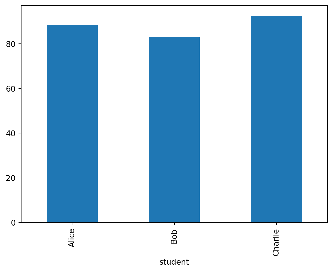

`groupby()` Summary

The groupby() function is essential for:

Calculating statistics by category
Finding patterns in subgroups
Data aggregation and summarization
Feature engineering (with transform)
Comparative analysis

Master the split-apply-combine pattern, and you’ll unlock powerful data analysis capabilities!

`groupby()` Practice Exercise

Try this on your own:

# Create sample data
practice_data = {
    'department': ['Sales', 'Sales', 'IT', 'IT', 'HR', 'HR', 'Sales', 'IT'],
    'employee': ['John', 'Jane', 'Bob', 'Alice', 'Tom', 'Mary', 'Steve', 'Linda'],
    'salary': [50000, 55000, 65000, 70000, 48000, 52000, 53000, 68000],
    'experience': [2, 3, 5, 7, 1, 4, 3, 6]
}

practice_df = pd.DataFrame(practice_data)

# Try to answer:
# 1. What's the average salary by department?
# 2. What's the total experience and max salary by department?
# 3. Add a column showing each employee's salary as a percentage of their department's total?

Other Pandas Classes

A DataFrame is essentially an annotated 2-D array.

Pandas also has annotated versions of 1-D and 3-D arrays.

A 1-D array in Pandas is called a Series. You can think of DataFrames as a dictionary of Series.

A 3-D array in Pandas is created using a MultiIndex.

For more information read the documentation.

In Class Activity

Iris Flower Analysis with Pandas

Duration: 20-25 minutes | Teams: 3 students each

Dataset: Iris Flower Dataset

Download Instructions: The Iris dataset is built into seaborn, so no download needed!

import pandas as pd
import seaborn as sns

# Load the Iris dataset directly
iris = sns.load_dataset('iris')

Team Roles (2 minutes)

Data Loader: Loads data and explores structure
Data Analyzer: Performs calculations and filtering
Data Visualizer: Creates plots and charts

Activity Tasks (20 minutes)

Phase 1: Data Loading & Exploration (5 minutes) 1. Check the shape and column names 2. Use .head(), .info(), and .describe() to explore the data


# Replace 0 and '[]' with the correct methods on iris
print(f"Dataset shape: {0}")
print(f"Columns: {['']}")

# Look at the first few rows
print("First 5 rows:")

# Get basic info about the dataset
print("\nDataset Info:")

# Describe the dataset with summary statistics
print("\nSummary Statistics:")

Phase 2: Basic Data Manipulation (8 minutes) 1. Create new columns: - Add a ‘petal_area’ column (petal_length × petal_width) - Create a ‘sepal_area’ column (sepal_length × sepal_width) - Create a ‘size_category’ column: - ‘Small’ (petal_area < 2) - ‘Medium’ (petal_area 2-5) - ‘Large’ (petal_area > 5)

# Create petal area column
iris['petal_area'] = ...

# Create sepal area column
iris['sepal_area'] = ...

# Create size category column
def categorize_size(petal_area):
    if ... :
        return 'Small'
    elif ... :
        return 'Medium'
    else:
        return 'Large'

iris['size_category'] = ...

print("New columns created:")
print(iris[['petal_length', 'petal_width', 'petal_area', 'size_category']].head(10))

Data Filtering:
- Find all ‘setosa’ species flowers
- Filter for large flowers only
- Find flowers with sepal_length > 6

# Find all 'setosa' species flowers
setosa_flowers = ...
print(f"Setosa flowers: {len(setosa_flowers)} out of {len(iris)}")

# Filter for large flowers only
large_flowers = ...
print(f"Large flowers: {len(large_flowers)} out of {len(iris)}")

# Find flowers with sepal_length > 6
long_sepal = ...
print(f"Flowers with sepal_length > 6: {len(long_sepal)} out of {len(iris)}")

Basic Analysis:
- Count flowers by species
- Find average petal length by species

# Count flowers by species
species_counts = ...
print("Flowers by species:")
print(species_counts)

# Find average petal length by species
avg_petal_by_species = ...
print("\nAverage petal length by species:")
print(avg_petal_by_species)

Phase 3: Simple Visualizations (7 minutes) 1. Create 2-3 basic plots: - Histogram of petal length - Bar chart of flower count by species - Scatter plot: sepal_length vs sepal_width

# Create a figure with subplots
fig, axes = plt.subplots(2, 2, figsize=(15, 10))

# 1. Histogram of petal length
axes[0, 0].hist(iris['petal_length'], bins=15, alpha=0.7, edgecolor='black', color='skyblue')
axes[0, 0].set_title('Distribution of Petal Length')
axes[0, 0].set_xlabel('Petal Length (cm)')
axes[0, 0].set_ylabel('Frequency')
axes[0, 0].grid(True, alpha=0.3)

# 2. Bar chart of flower count by species
species_counts = iris['species'].value_counts()
species_counts.plot(kind='bar', ax=axes[0, 1], color=['red', 'green', 'blue'])
axes[0, 1].set_title('Number of Flowers by Species')
axes[0, 1].set_xlabel('Species')
axes[0, 1].set_ylabel('Number of Flowers')
axes[0, 1].tick_params(axis='x', rotation=45)
axes[0, 1].grid(True, alpha=0.3)

# 3. Scatter plot: sepal_length vs sepal_width
for species in iris['species'].unique():
    data = iris[iris['species'] == species]
    axes[1, 0].scatter(data['sepal_length'], data['sepal_width'], 
                      alpha=0.7, label=species, s=50)
axes[1, 0].set_title('Sepal Length vs Sepal Width (by Species)')
axes[1, 0].set_xlabel('Sepal Length (cm)')
axes[1, 0].set_ylabel('Sepal Width (cm)')
axes[1, 0].legend()
axes[1, 0].grid(True, alpha=0.3)

# 4. Bar chart of size categories (if size_category column exists)
if 'size_category' in iris.columns:
    size_categories = iris['size_category'].value_counts()
    size_categories.plot(kind='bar', ax=axes[1, 1], color=['orange', 'lightgreen', 'lightcoral'])
    axes[1, 1].set_title('Flowers by Size Category')
    axes[1, 1].set_xlabel('Size Category')
    axes[1, 1].set_ylabel('Number of Flowers')
    axes[1, 1].tick_params(axis='x', rotation=0)
    axes[1, 1].grid(True, alpha=0.3)
else:
    # Alternative: petal length vs petal width scatter
    axes[1, 1].scatter(iris['petal_length'], iris['petal_width'], alpha=0.7, s=50)
    axes[1, 1].set_title('Petal Length vs Petal Width')
    axes[1, 1].set_xlabel('Petal Length (cm)')
    axes[1, 1].set_ylabel('Petal Width (cm)')
    axes[1, 1].grid(True, alpha=0.3)

plt.tight_layout()
plt.show()

Upon Completion:

Execute all the cells, save and download the notebook and submit to Gradescope.

Recap

In this section we got a first glimpse of the Pandas library.

We learned how to:

load data from a CSV file
inspect the data
manipulate the data
plot the data
access rows and columns of the dataframe
filter the data
create new columns
group the data

Introduction

Pandas

Fetching, storing and retrieving your data

Writing/Reading to/from a .csv file

Working with data columns

A sampling of DataFrame methods.

Plotting methods

Accessing rows of the DataFrame

Filtering

Creating new columns

Understanding pandas DataFrame.groupby()

Introduction

Basic Concept

Example 1: Simple Grouping

Example 2: Multiple Aggregations

Example 3: Grouping by Multiple Columns

Example 4: Aggregating Multiple Columns

Example 5: Different Aggregations for Different Columns

Example 6: Using Custom Functions

Example 7: Filtering Groups

Example 8: Transform - Keeping Original Shape

Example 9: Apply - Maximum Flexibility

Example 10: Iterating Over Groups

Common Aggregation Functions

Example 11: (Synthetic) Sales Data Analysis

Tips and Best Practices

Visualizing Grouped Data

groupby() Summary

groupby() Practice Exercise

Other Pandas Classes

In Class Activity

Iris Flower Analysis with Pandas

Dataset: Iris Flower Dataset

Team Roles (2 minutes)

Activity Tasks (20 minutes)

Recap

Writing/Reading to/from a `.csv` file

`groupby()` Summary

`groupby()` Practice Exercise