Matrix Factorization Techniques for Recommender Systems, (Koren et al. 2009)
Collaborative Filtering with Temporal Dynamics, (Koren 2009)
What are Recommender Systems?
The concept of recommender systems emerged in the late 1990s / early 2000s as social life moved online:
online purchasing and commerce
online discussions and ratings
social information sharing
In these systems the amount of content was exploding and users were having a hard time finding things they were interested in.
Users wanted recommendations.
Over time, the problem has only gotten worse:
An enormous need has emerged for systems to help sort through products, services, and content items.
This often goes by the term personalization.
Some examples (as of Fall 2024):
Movie recommendation (Netflix ~6.5K movies and shows, YouTube ~14B videos)
Related product recommendation (Amazon ~600M products)
Web page ranking (Google >>100B pages)
Social content filtering (Facebook, Twitter)
Services (Airbnb, Uber, TripAdvisor)
News content recommendation (Apple News)
Priority inbox & spam filtering (Gmail)
Online dating (Match.com)
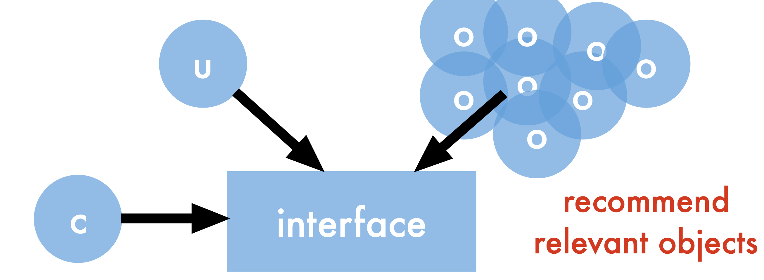
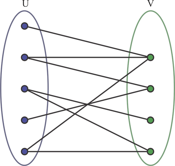
A more formal view:
User - requests content
Objects - instances of content
Context - ratings, purchases, views, device, location, time, history
Interface - browser, mobile
Inferring Preferences
Unfortunately, users generally have a hard time explaining what types of content they prefer.
Some early systems worked by interviewing users to ask what they liked. Those systems did not work very well.
A very interesting article about the earliest personalization systems is User Modeling via Stereotypes by Elaine Rich, dating from 1979.
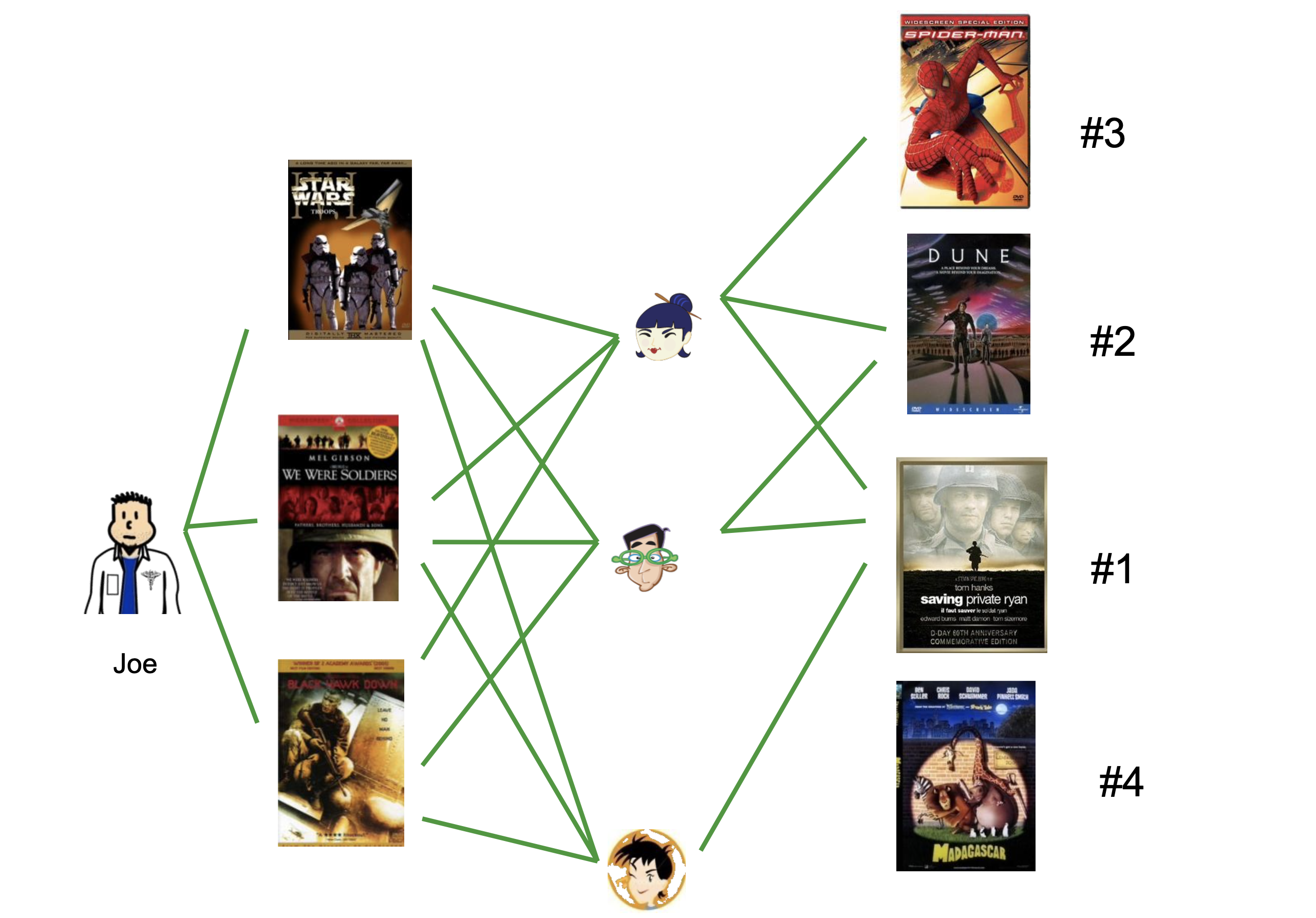
Instead, modern systems work by capturing user’s opinions about specific items.
This can be done actively:
When a user is asked to rate a movie, product, or experience,
or it can be done passively:
By noting which items a user chooses to purchase (for example).
Challenges
The biggest issue is scalability: typical data for this problem is huge.
Millions of objects
100s of millions of users
Changing user base
Changing inventory (movies, stories, goods)
Available features
Imbalanced dataset
User activity / item reviews are power law distributed
This data is a subset of the data presented in: “From amateurs to connoisseurs: modeling the evolution of user expertise through online reviews,” by J. McAuley and J. Leskovec. WWW, 2013
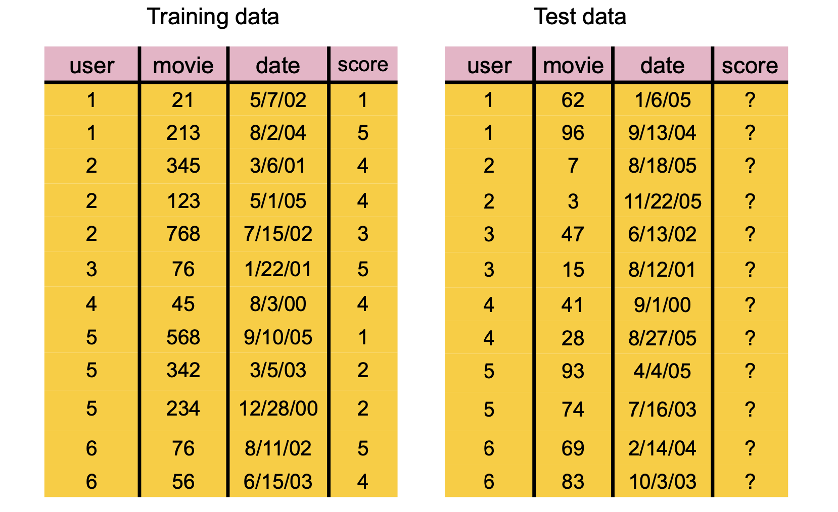
Example
Let’s look at a dataset for testing recommender systems consisting of Amazon movie reviews:
We’ll download a compressed pickle file containing the data if it is not already present.
Code
# This is a 647 MB file, delete it after useimport gdownurl ="https://drive.google.com/uc?id=14GakA7oOjbQp7nxcGApI86WlP3GrYTZI"pickle_output ="train.pkl.gz"import os.pathifnot os.path.exists(pickle_output): gdown.download(url, pickle_output)
HelpfulnessNumerator: The number of users who found the review helpful (the “yes” votes)
HelpfulnessDenominator: The total number of users who voted on whether the review was helpful (both “yes” and “no” votes)
Now we can count the number of users and movies:
Code
from IPython.display import display, Markdownn_users = df["UserId"].unique().shape[0]n_movies = df["ProductId"].unique().shape[0]n_reviews =len(df)display(Markdown(f'There are:\n'))display(Markdown(f'* {n_reviews:,} reviews\n* {n_movies:,} movies\n* {n_users:,} users'))display(Markdown(f'There are {n_users * n_movies:,} potential reviews, meaning sparsity of {(n_reviews/(n_users * n_movies)):0.4%}'))
There are:
1,697,533 reviews
50,052 movies
123,960 users
There are 6,204,445,920 potential reviews, meaning sparsity of 0.0274%
where
\[
\text{sparsity}
= \frac{\text{\# of reviews}}{\text{\# of users} \times \text{\# of movies}}
= \frac{\text{\# of reviews}}{\text{\# of potential reviews}}
\]
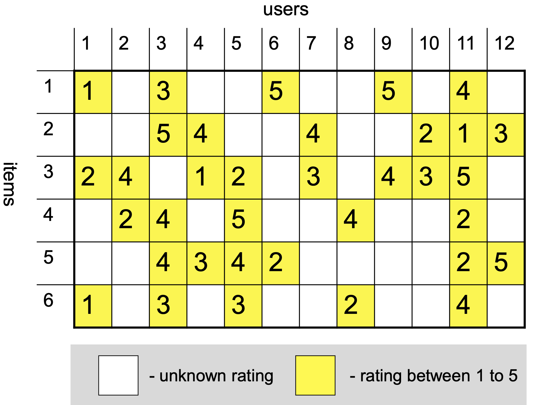
Reviews are Sparse
Only 0.02% of the reviews are available – 99.98% of the reviews are missing.
Code
display(Markdown(f'There are on average {n_reviews/n_movies:0.1f} reviews per movie'+f' and {n_reviews/n_users:0.1f} reviews per user'))
There are on average 33.9 reviews per movie and 13.7 reviews per user
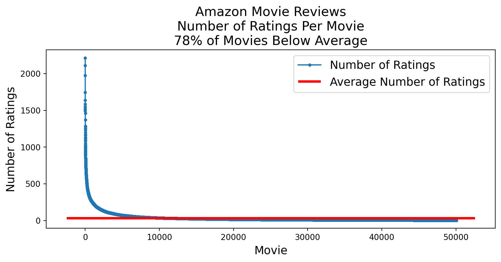
Sparseness is Skewed
Although on average a movie receives 34 reviews, almost all movies have even fewer reviews.
Code
plt.figure(figsize=(10, 4)) # Set the figure sizereviews_per_movie = df.groupby('ProductId').count()['Id'].valuesfrac_below_mean = np.sum(reviews_per_movie < (n_reviews/n_movies))/len(reviews_per_movie)plt.plot(sorted(reviews_per_movie, reverse=True), '.-')xmin, xmax, ymin, ymax = plt.axis()plt.hlines(n_reviews/n_movies, xmin, xmax, 'r', lw =3)plt.ylabel('Number of Ratings', fontsize =14)plt.xlabel('Movie', fontsize =14)plt.legend(['Number of Ratings', 'Average Number of Ratings'], fontsize =14)plt.title(f'Amazon Movie Reviews\nNumber of Ratings Per Movie\n'+f'{frac_below_mean:0.0%} of Movies Below Average', fontsize =16);
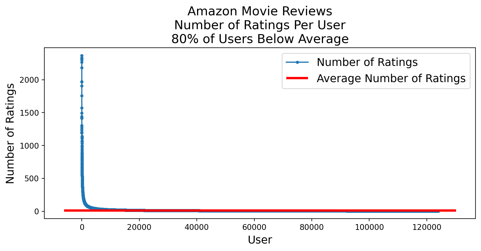
Likewise, although the average user writes 14 reviews, almost all users write even fewer reviews.
Code
plt.figure(figsize=(10, 4)) # Set the figure sizereviews_per_user = df.groupby('UserId').count()['Id'].valuesfrac_below_mean = np.sum(reviews_per_user < (n_reviews/n_users))/len(reviews_per_user)plt.plot(sorted(reviews_per_user, reverse=True), '.-')xmin, xmax, ymin, ymax = plt.axis()plt.hlines(n_reviews/n_users, xmin, xmax, 'r', lw =3)plt.ylabel('Number of Ratings', fontsize =14)plt.xlabel('User', fontsize =14)plt.legend(['Number of Ratings', 'Average Number of Ratings'], fontsize =14)plt.title(f'Amazon Movie Reviews\nNumber of Ratings Per User\n'+f'{frac_below_mean:0.0%} of Users Below Average', fontsize =16);
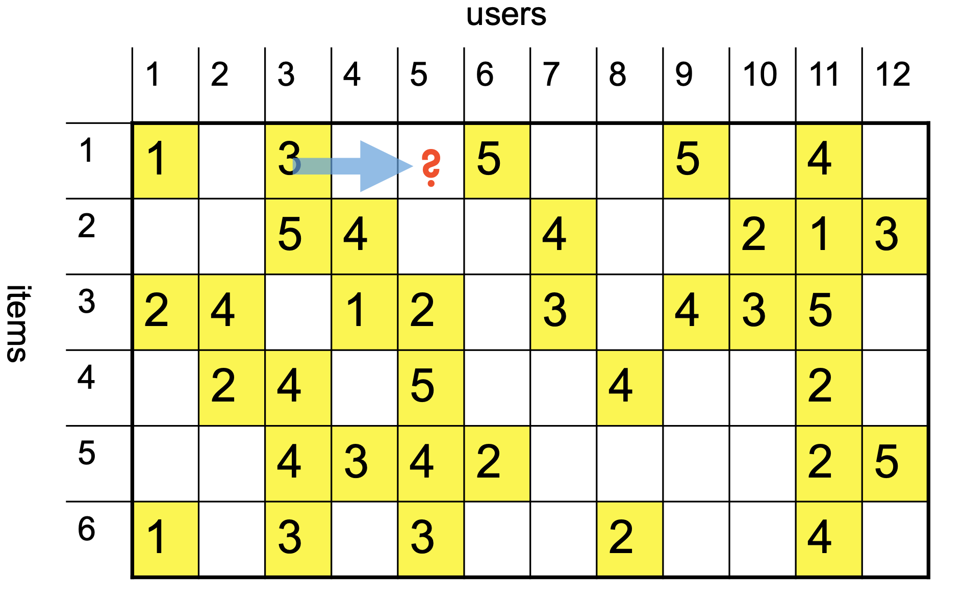
Objective Function
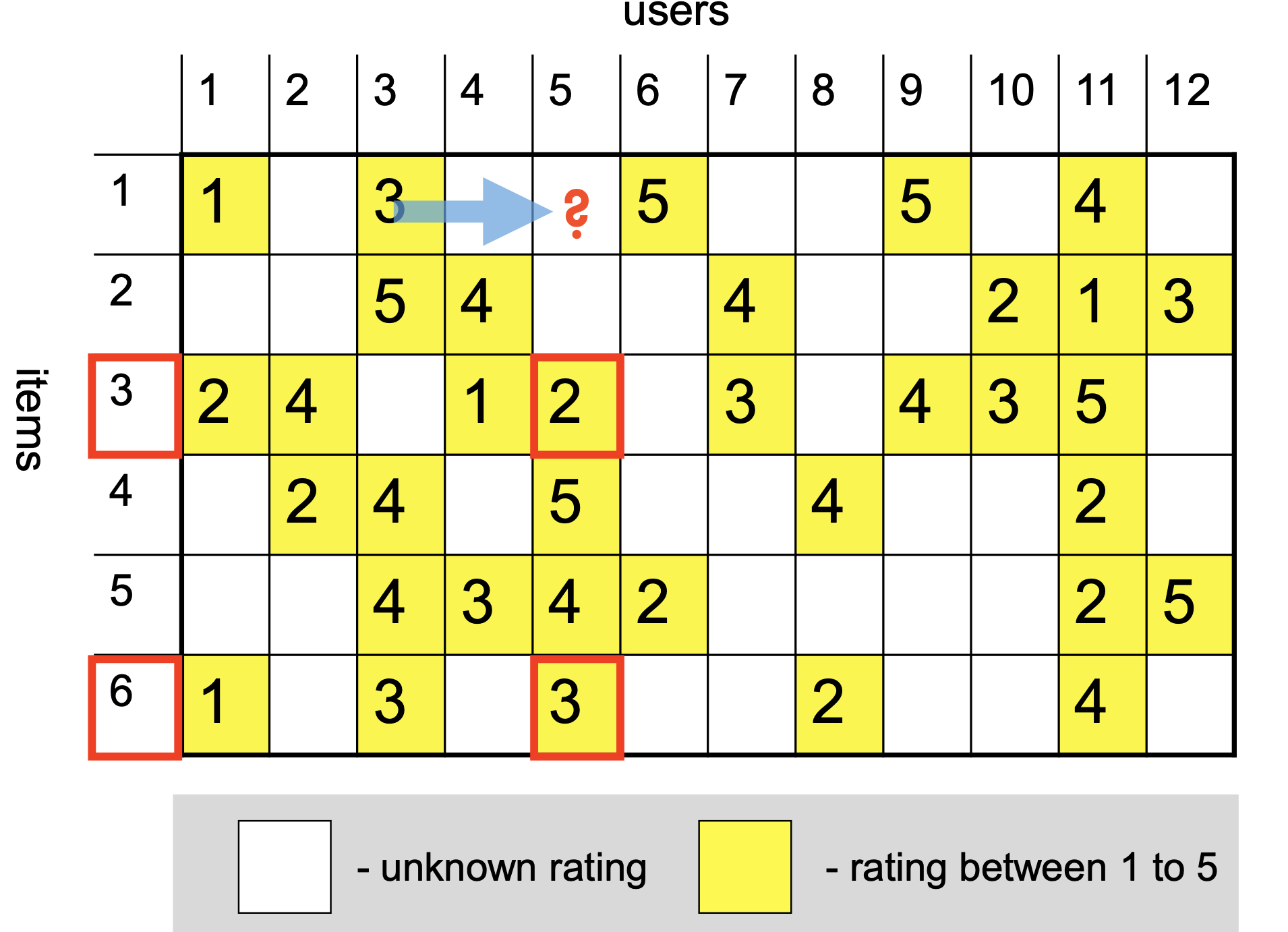
Ultimately, our goal is to predict the rating that a user would give to an item.
For that, we need to define a loss or objective function.
A typical objective function is root mean square error (RMSE)
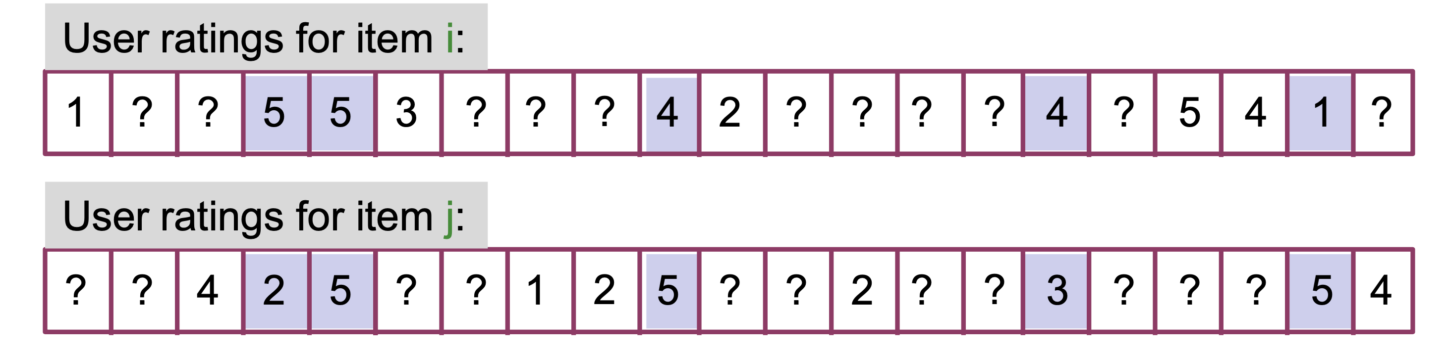
# Create new lists where only numbers are kept that are not np.nan in both listsfiltered_ratings_item_i = [rating_i for rating_i, rating_j inzip(ratings_item_i, ratings_item_j) ifnot np.isnan(rating_i) andnot np.isnan(rating_j)]filtered_ratings_item_j = [rating_j for rating_i, rating_j inzip(ratings_item_i, ratings_item_j) ifnot np.isnan(rating_i) andnot np.isnan(rating_j)]display(Markdown(f'Common ratings for item $i$: {filtered_ratings_item_i}'))display(Markdown(f'Common ratings for item $j$: {filtered_ratings_item_j}'))
Common ratings for item \(i\): [5, 5, 4, 4, 1]
Common ratings for item \(j\): [2, 5, 5, 3, 5]
Example, continued
Code
display(Markdown(f'Common ratings for item $i$: {filtered_ratings_item_i}'))display(Markdown(f'Common ratings for item $j$: {filtered_ratings_item_j}'))
Common ratings for item \(i\): [5, 5, 4, 4, 1]
Common ratings for item \(j\): [2, 5, 5, 3, 5]
Now we can compute the Pearson correlation coefficient:
Which is a moderate negative correlation, meaning that as item \(i\) gets rated higher, item \(j\) gets rated lower.
Pearson Correlation Coefficient
The Pearson correlation coefficient, often denoted as \(r\), is a measure of the linear correlation between two variables \(X\) and \(Y\). It quantifies the degree to which a linear relationship exists between the variables. The value of \(r\) ranges from -1 to 1, where:
\(r = 1\) indicates a perfect positive linear relationship,
\(r = -1\) indicates a perfect negative linear relationship,
\(r = 0\) indicates no linear relationship.
The formula for the Pearson correlation coefficient is:
Where: - \(X_i\) and \(Y_i\) are the individual sample points, - \(\bar{X}\) and \(\bar{Y}\) are the means of the \(X\) and \(Y\) samples, respectively.
The Pearson correlation coefficient is sensitive to outliers and assumes that the relationship between the variables is linear and that the data is normally distributed.
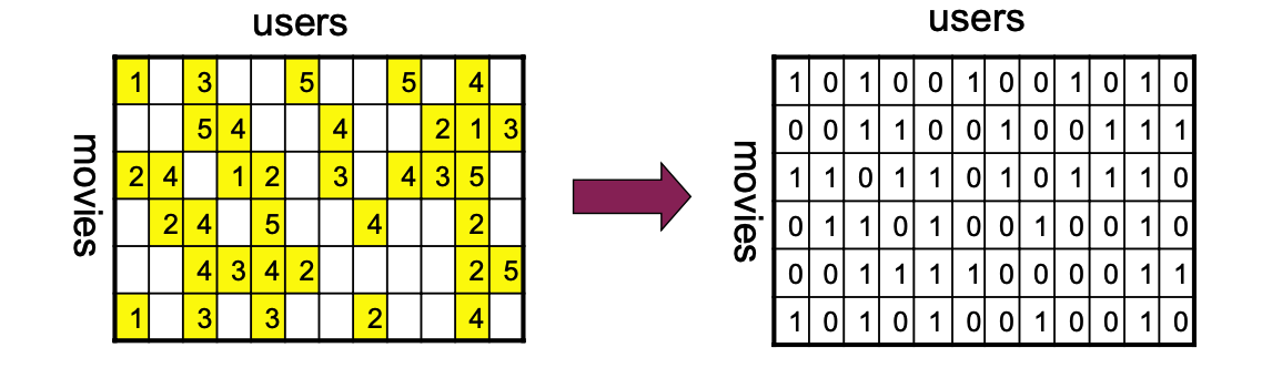
Similarity for Binary Data
In some cases we will need to work with binary \(r_{ui}\).
For example, purchase histories on an e-commerce site, or clicks on an ad.
In this case, an appropriate replacement for Pearson \(r\) is the Jaccard similarity coefficient or Intersection over Union.
Here \(i \in R(u)\) means the set of items rated by user \(u\) and \(u \in R(i)\) means the set of users who have rated item \(i\) and \(|R(u)|\) is the number of ratings.
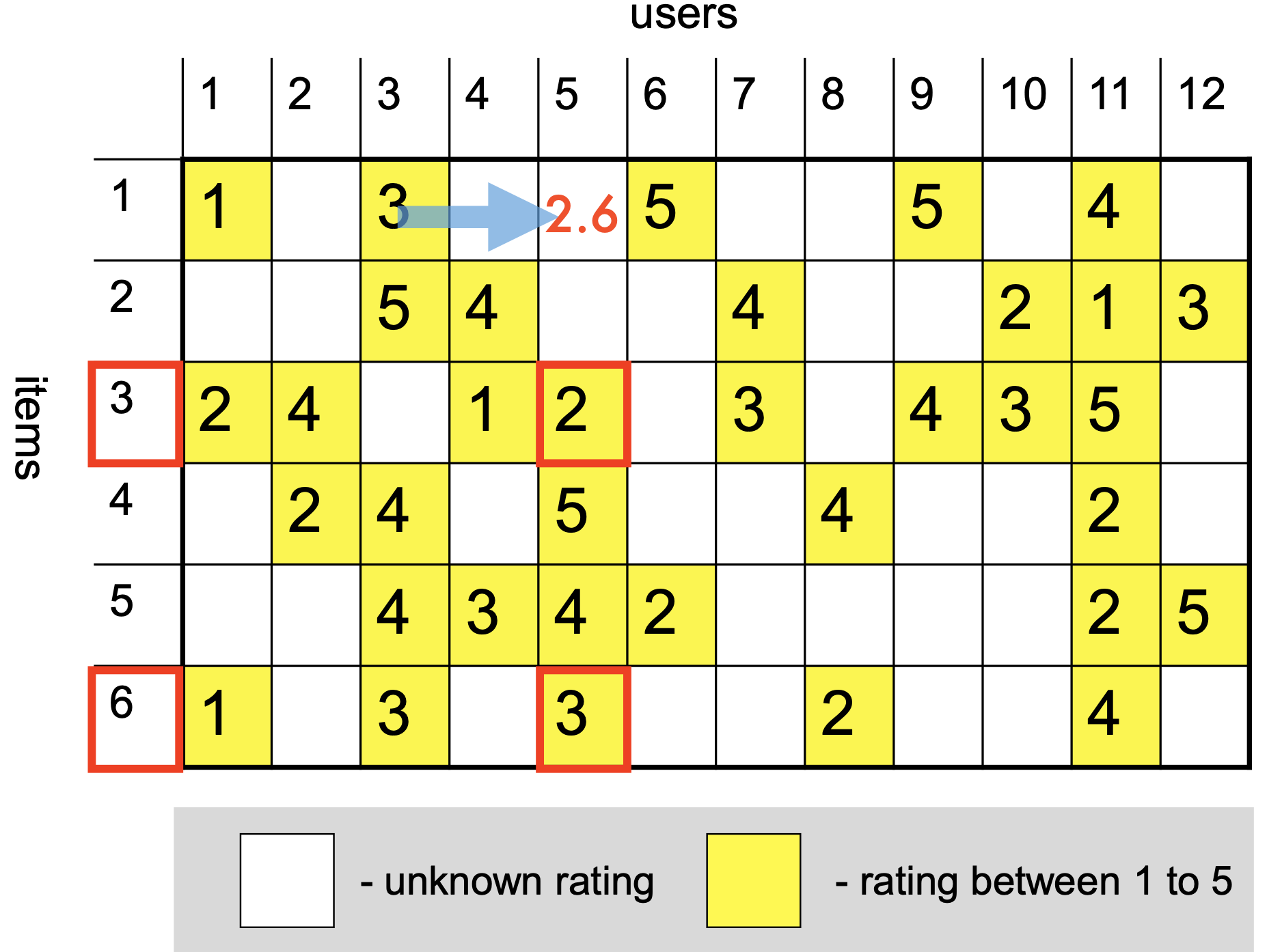
Now that we have learned the biases, we can do a better job of estimating correlation:
When \(s_{ij}\) is negative (negative correlation), here’s what happens:
Numerator: The term \(s_{ij}(r_{uj} - b_{uj})\) becomes negative when \(s_{ij} < 0\). This means:
If user \(u\) rated item \(j\)above its bias (\(r_{uj} - b_{uj} > 0\)), the negative similarity will push the prediction for item \(i\)down
If user \(u\) rated item \(j\)below its bias (\(r_{uj} - b_{uj} < 0\)), the negative similarity will push the prediction for item \(i\)up
This makes intuitive sense: if items \(i\) and \(j\) are negatively correlated, then liking one means you’re likely to dislike the other.
Denominator: When \(s_{ij}\) is negative, it contributes a negative value to the sum in the denominator. This can potentially lead to issues:
If all similarities are negative, the denominator becomes negative
If there’s a mix of positive and negative similarities, they might partially cancel out, potentially making the denominator close to zero or even zero
Common Solutions
To address these issues, practitioners typically use one of these approaches:
Use only positive similarities: Filter out items with negative correlation (only use \(k\)-NN where \(s_{ij} > 0\))
Use absolute values in denominator: \(\displaystyle\hat{r}_{ui} = b_{ui} + \frac{\sum_{j \in n_k(i, u)} s_{ij}(r_{uj} - b_{uj})}{\sum_{j \in n_k(i, u)} |s_{ij}|}\)
Shift and scale similarities: Transform correlation values from \([-1, 1]\) to \([0, 1]\) using \(s'_{ij} = \frac{s_{ij} + 1}{2}\)
The first approach (filtering to positive similarities) is most common because negatively correlated items are typically less informative for prediction than positively correlated items in most domains.
Assessing CF
This completes the high level view of CF.
Working with user-user similarities is analogous.
Strengths:
Essentially no training.
The reliance on \(k\)-nearest neighbors helps in this respect.
Easy to update with new users, items, and ratings.
Explainable:
“We recommend Minority Report because you liked Blade Runner and Total Recall.”
Weaknesses:
Accuracy can be a problem – resulting in poor recommendations
Scalability can be a problem – compute grows (think \(k\)-NN)
Matrix Factorization Approaches
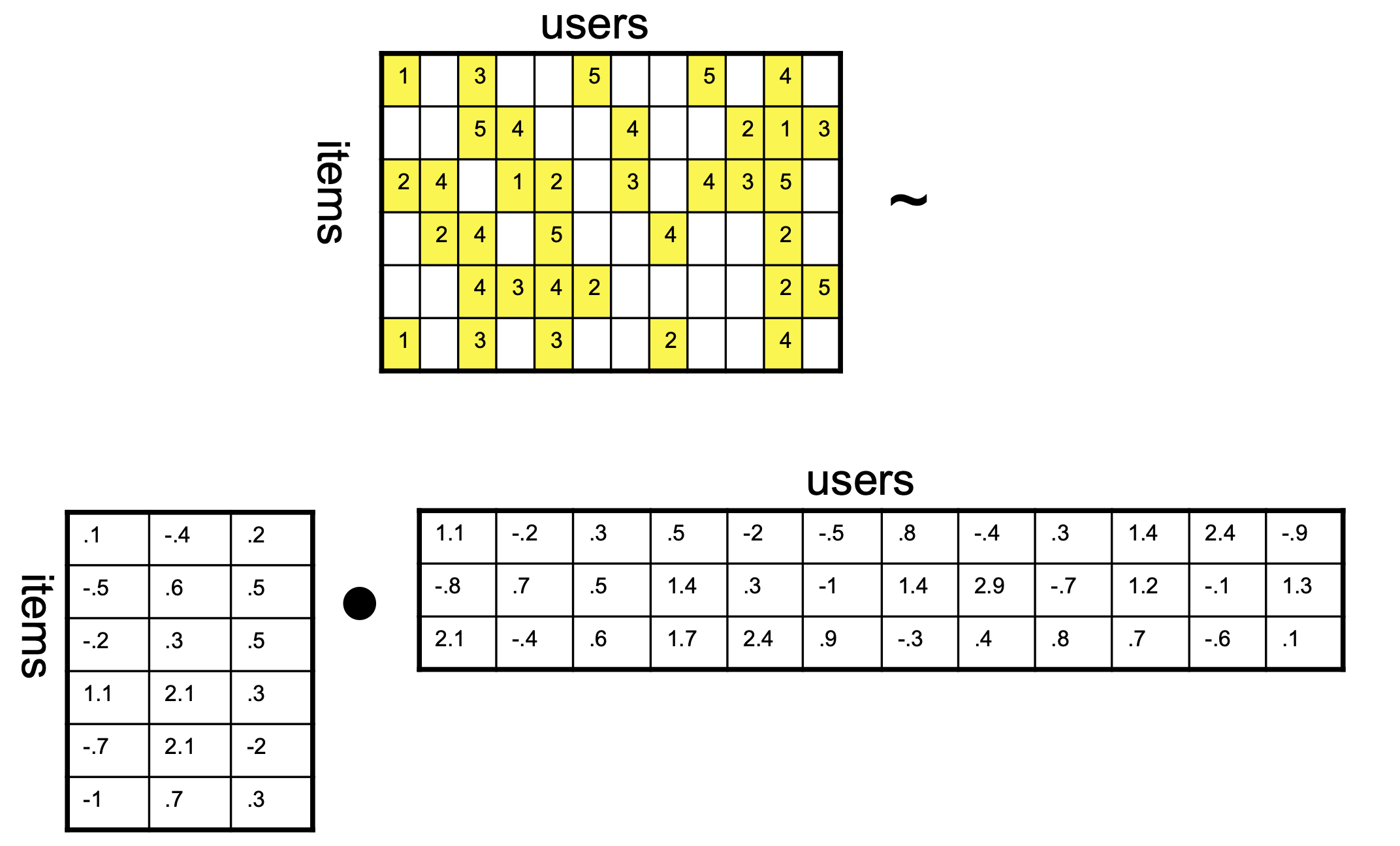
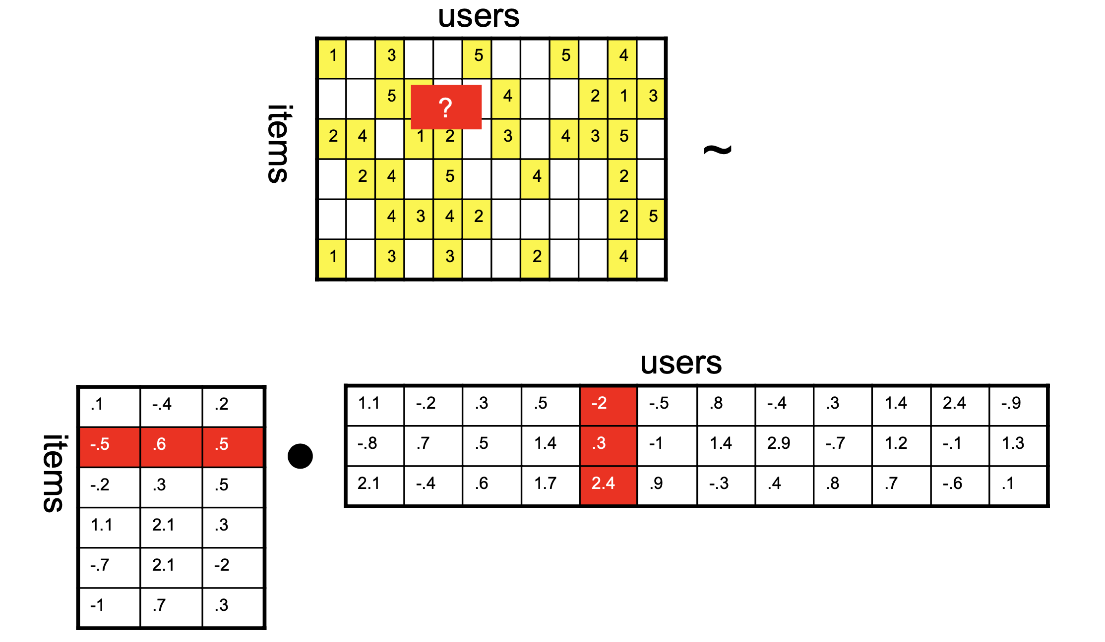
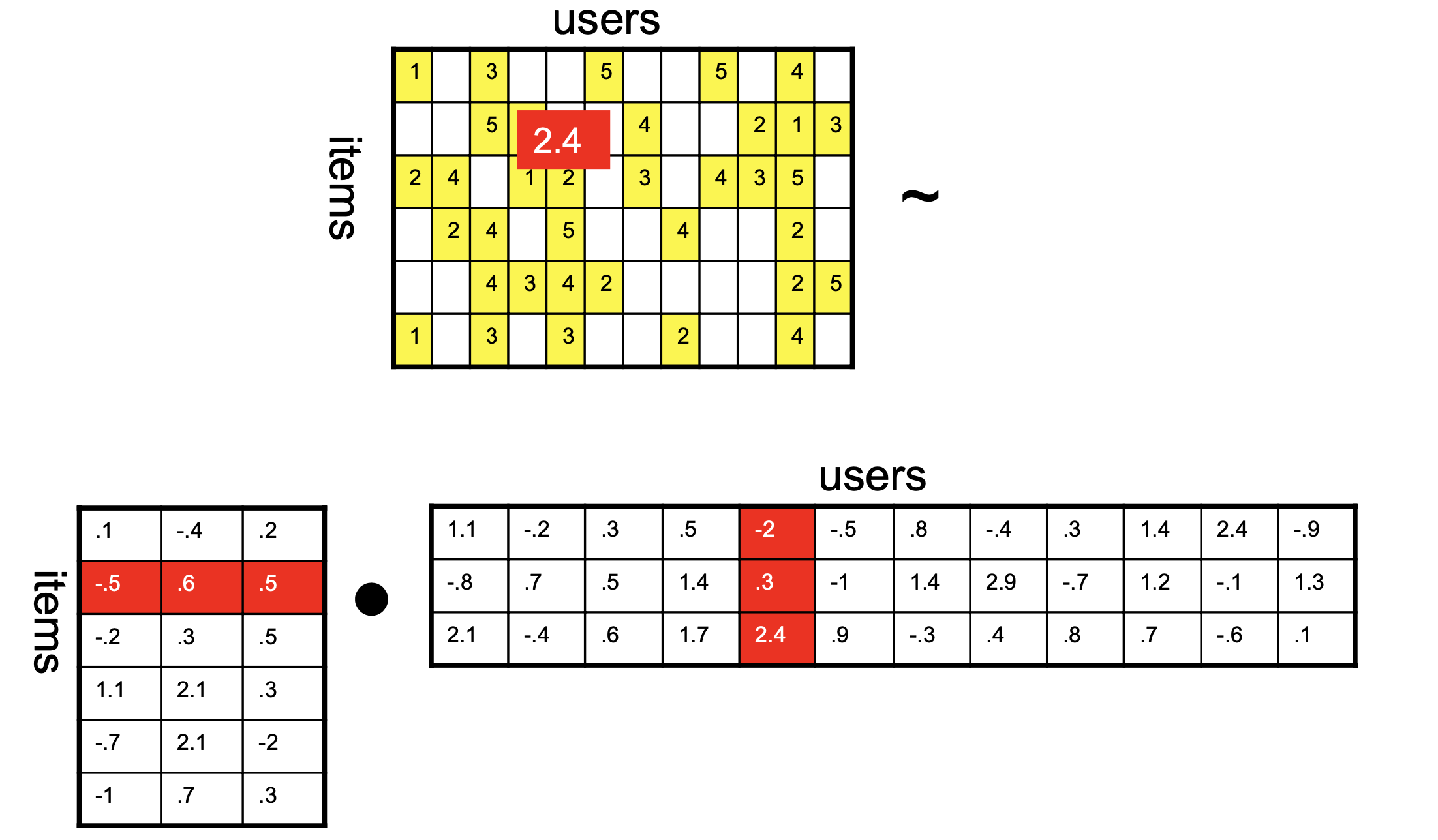
Matrix Factorization
Note that standard CF forces us to consider similarity among items, or among users, but does not take into account both.
Can we use both kinds of similarity simultaneously?
We can’t use both the rows and columns of the ratings matrix \(R\) at the same time – the user and item vectors live in different vector spaces.
\(k\) is the rank of the factorization and dimensionality of the latent space.
The \((\cdot)_S\) notation means that we are only considering the subset of matrix entries that correspond to known reviews (the set \(S\)).
Note that as usual, we add \(\ell_2\) penalization to avoid overfitting (Ridge regression).
Once again, this problem is jointly convex in that it is convex in each of the variables \(U\) and \(V\).
In particular, if we hold either \(U\) or \(V\) constant, then the result is a simple ridge regression.
So one commonly used algorithm for this problem is called alternating least squares (ALS):
Hold \(U\) constant, and solve for \(V\)
Hold \(V\) constant, and solve for \(U\)
If not converged, go to Step 1.
The only thing we’ve left out at this point is how to deal with the missing entries of \(R\).
It’s not hard, but the details aren’t that interesting, so we’ll give you code instead!
ALS in Practice
The entire Amazon reviews dataset is too large to work with easily, and it is too sparse.
Hence, we will take the densest rows and columns of the matrix.
Code
# print(df.shape)# The densest columns: products with more than 50 reviewspids = df.groupby('ProductId').count()['Id']hi_pids = pids[pids >50].index# reviews that are for these productshi_pid_rec = [r in hi_pids for r in df['ProductId']]# the densest rows: users with more than 50 reviewsuids = df.groupby('UserId').count()['Id']hi_uids = uids[uids >50].index# reviews that are from these usershi_uid_rec = [r in hi_uids for r in df['UserId']]# The result is a list of booleans equal to the number of rewviews# that are from those dense users and moviesgoodrec = [a and b for a, b inzip(hi_uid_rec, hi_pid_rec)]
Now we create a \(\textnormal{UserID} \times \textnormal{ProductID}\) matrix from these reviews.
# Import local python package MF.pyimport recommender_MF as MF# Instantiate the model# We are pulling these hyperparameters out of the air -- that's not the right way to do it!RS = MF.als_MF(rank =20, lambda_ =1)
%time pred, error = RS.fit_model(R)
CPU times: user 24.3 s, sys: 176 ms, total: 24.5 s
Wall time: 24.4 s
print(f'RMSE on visible entries (training data): {np.sqrt(error/R.count().sum()):0.3f}')
RMSE on visible entries (training data): 0.343
And we can look at a small part of the predicted ratings matrix and see that it is a dense matrix:
Code
print(f'Shape of predicted ratings matrix: {pred.shape}')pred.iloc[900:905, 1000:1004]
Shape of predicted ratings matrix: (3677, 7244)
ProductId
1417024917
1417030321
1417030976
1417054069
UserId
A1WLZYEOIL1HLT
3.374718
4.104916
4.219042
5.402325
A1WNJVA59HLMO5
3.470308
5.736709
5.306202
4.309822
A1WR12AC35R3K6
4.007515
4.262276
4.590415
3.147474
A1WSFHRBY2ZD1R
4.030337
4.484953
3.857923
5.263364
A1WUMTJOASEL5F
2.818730
3.302549
4.571714
5.893641
Code
## todo: hold out test data, compute oos error# We create a mask of the known entries, then calculate the indices of the known# entries, then split that data into training and test sets.# Create a mask for the known entriesRN =~R.isnull()# Get the indices of the known entriesvisible = np.where(RN)# Split the data into training and test setsimport sklearn.model_selection as model_selectionX_train, X_test, Y_train, Y_test = model_selection.train_test_split(visible[0], visible[1], test_size =0.1)
Just for comparison’s sake, let’s check the performance of \(k\)-NN on this dataset.
Again, this is only on the training data – so overly optimistic for sure.
And note that this is a subset of the full dataset – the subset that is “easiest” to predict due to density.
Code
from sklearn.neighbors import KNeighborsRegressorfrom sklearn.metrics import mean_squared_error# Drop the columns that are not featuresX_train = good_df.drop(columns=['Id', 'ProductId', 'UserId', 'Text', 'Summary'])# The target is the scorey_train = good_df['Score']# Using k-NN on features HelpfulnessNumerator, HelpfulnessDenominator, Score, Timemodel = KNeighborsRegressor(n_neighbors=3).fit(X_train, y_train)%time y_hat = model.predict(X_train)
CPU times: user 296 ms, sys: 6.38 ms, total: 302 ms
Wall time: 304 ms
Code
print(f'RMSE on visible entries (test set): {np.sqrt(mean_squared_error(y_train, y_hat)):.3f}')
RMSE on visible entries (test set): 0.494
Assessing Matrix Factorization
Matrix Factorization per se is a good idea.
However, many of the improvements we’ve discussed for CF apply to MF as well.
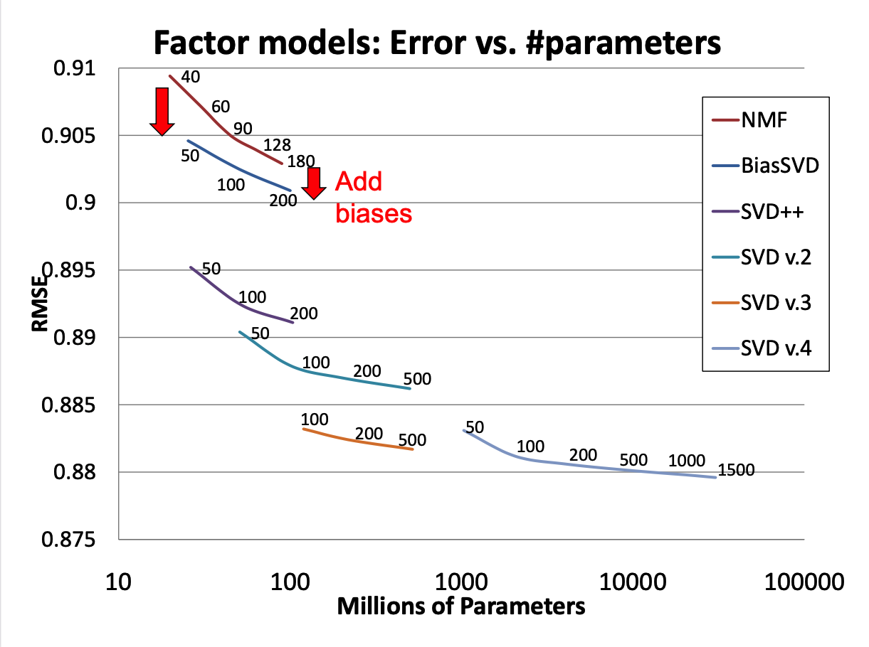
To illustrate, we’ll look at some of the successive improvements used by the team that won the Netflix prize (“BellKor’s Pragmatic Chaos”).
When the prize was announced, the Netflix supplied solution achieved an RMSE of 0.951.
By the end of the competition (about 3 years), the winning team’s solution achieved RMSE of 0.856.
Let’s restate our MF objective in a way that will make things clearer:
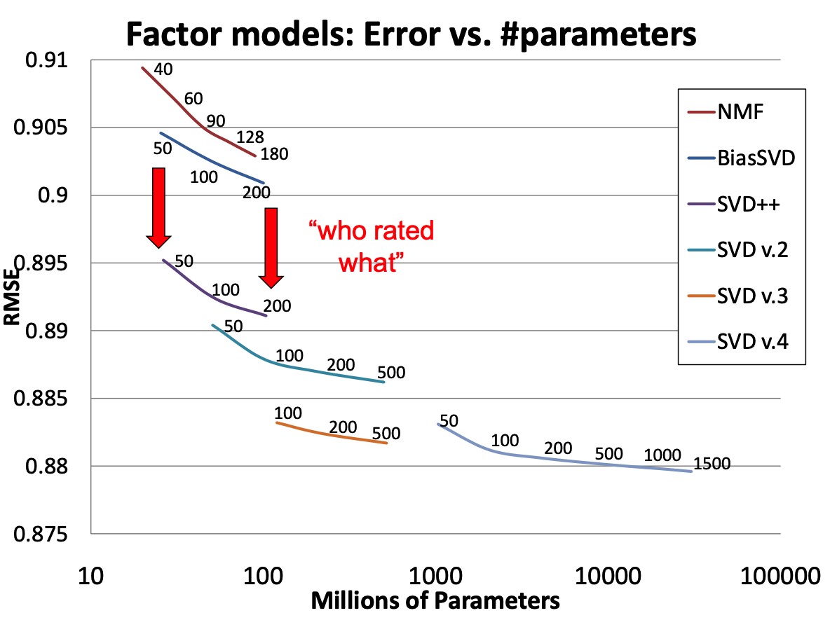
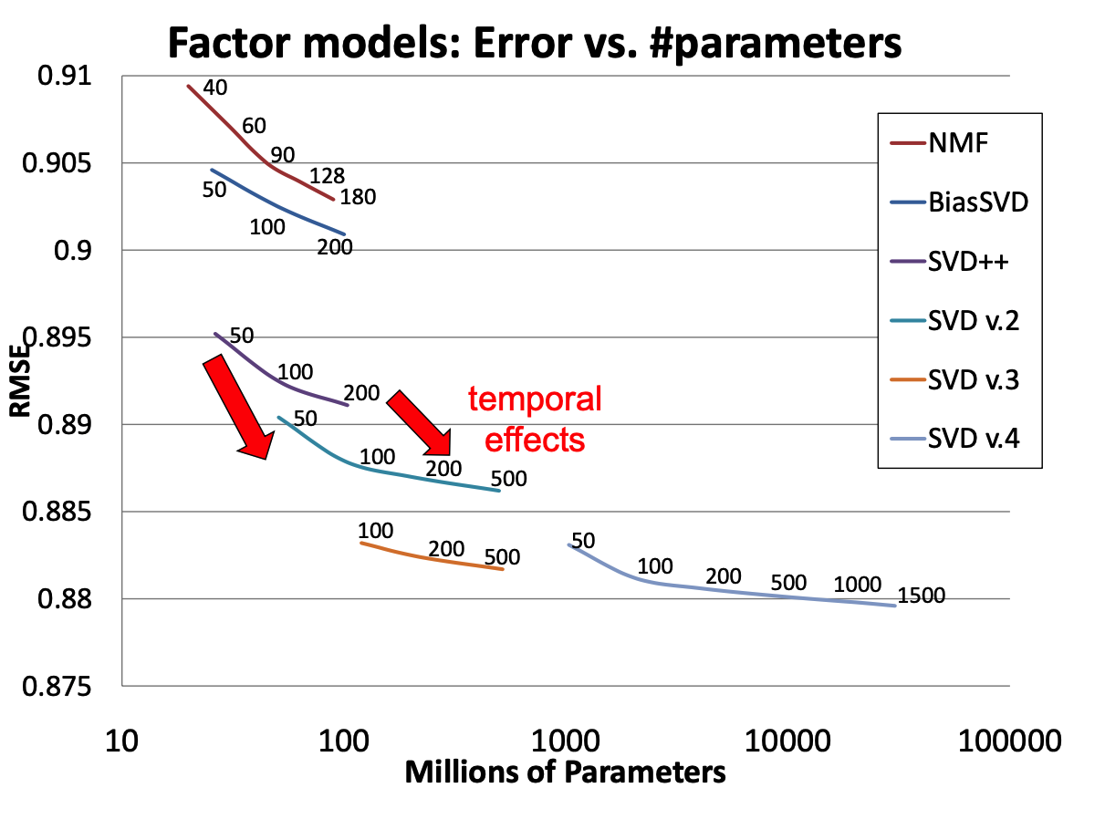
Figure 2: Matrix factorization models’ accuracy. The plots show the root-mean-square error of each of four individual factor models (lower is better). Accuracy improves when the factor model’s dimensionality (denoted by numbers on the charts) increases. In addition, the more refined factor models, whose descriptions involve more distinct sets of parameters, are more accurate.
2. Who Rated What?
In reality, ratings are not provided at random.
Take note of which users rated the same movies (ala CF) and use this information.
To estimate these billions of parameters, we cannot use alternating least squares or any linear algebraic method.
We need to use gradient descent (which we covered previously).
Recap
Introduction to recommender systems and their importance in modern society.
Explanation of collaborative filtering (CF) and its two main approaches: user-user similarity and item-item similarity.
Discussion on the challenges of recommender systems, including scalability and data sparsity.
Introduction to matrix factorization (MF) as an improvement over CF, using latent vectors and alternating least squares (ALS) for optimization.
Practical implementation of ALS for matrix factorization on a subset of Amazon movie reviews.
References
Koren, Yehuda. 2009. “Collaborative Filtering with Temporal Dynamics.”Proceedings of the 15th ACM SIGKDD International Conference on Knowledge Discovery and Data Mining 42: 447–56. https://dl.acm.org/doi/10.1145/1557019.1557072.
Koren, Yehuda, Robert Bell, and Chris Volinsky. 2009. “Matrix Factorization Techniques for Recommender Systems.”Computer 42 (8): 30–37. https://ieeexplore.ieee.org/document/5197422.
Naumov, Maxim et al. 2019. “Deep Learning Recommendation Model for Personalization and Recommendation Systems.”arXiv Preprint arXiv:1906.00091, May. http://arxiv.org/abs/1906.00091.