import numpy as npfrom sklearn.metrics.pairwise import cosine_similaritydef calculate_document_similarity():""" Calculate different similarity measures between two documents represented as word frequency vectors. """print("Document Similarity Analysis")print("="*40)# Given word frequency vectors doc_a = np.array([3, 2, 1, 0]) # [cat, dog, bird, fish] doc_b = np.array([1, 3, 0, 2]) # [cat, dog, bird, fish]print("Original word frequency vectors:")print(f"Document A: {doc_a} (cat: 3, dog: 2, bird: 1, fish: 0)")print(f"Document B: {doc_b} (cat: 1, dog: 3, bird: 0, fish: 2)")print()# Step 1: Convert to normalized vectors (divide by total word count) doc_a_normalized = doc_a / np.sum(doc_a) doc_b_normalized = doc_b / np.sum(doc_b)print("Step 1: Normalized vectors (divided by total word count)")print(f"Document A normalized: {doc_a_normalized}")print(f"Document B normalized: {doc_b_normalized}")print(f"Sum of normalized A: {np.sum(doc_a_normalized):.6f}")print(f"Sum of normalized B: {np.sum(doc_b_normalized):.6f}")print()# Step 2: Calculate cosine similarity# Reshape for sklearn's cosine_similarity function doc_a_reshaped = doc_a_normalized.reshape(1, -1) doc_b_reshaped = doc_b_normalized.reshape(1, -1) cosine_sim = cosine_similarity(doc_a_reshaped, doc_b_reshaped)[0][0]print("Step 2: Cosine similarity calculation")print(f"Cosine similarity: {cosine_sim:.6f}")print()# Manual calculation for verification dot_product = np.dot(doc_a_normalized, doc_b_normalized) norm_a = np.linalg.norm(doc_a_normalized) norm_b = np.linalg.norm(doc_b_normalized) cosine_sim_manual = dot_product / (norm_a * norm_b)print("Manual verification:")print(f"Dot product: {dot_product:.6f}")print(f"Norm of A: {norm_a:.6f}")print(f"Norm of B: {norm_b:.6f}")print(f"Cosine similarity (manual): {cosine_sim_manual:.6f}")print()# Step 3: Calculate dissimilarity dissimilarity =1- cosine_simprint("Step 3: Dissimilarity calculation")print(f"Dissimilarity (1 - cosine_similarity): {dissimilarity:.6f}")print()# Additional analysisprint("Additional Analysis:")print("-"*20)# Euclidean distance for comparison euclidean_dist = np.linalg.norm(doc_a_normalized - doc_b_normalized)print(f"Euclidean distance: {euclidean_dist:.6f}")# Manhattan distance manhattan_dist = np.sum(np.abs(doc_a_normalized - doc_b_normalized))print(f"Manhattan distance: {manhattan_dist:.6f}")print()return {'doc_a_normalized': doc_a_normalized,'doc_b_normalized': doc_b_normalized,'cosine_similarity': cosine_sim,'dissimilarity': dissimilarity,'euclidean_distance': euclidean_dist,'manhattan_distance': manhattan_dist }if__name__=="__main__": results = calculate_document_similarity()
Document Similarity Analysis
========================================
Original word frequency vectors:
Document A: [3 2 1 0] (cat: 3, dog: 2, bird: 1, fish: 0)
Document B: [1 3 0 2] (cat: 1, dog: 3, bird: 0, fish: 2)
Step 1: Normalized vectors (divided by total word count)
Document A normalized: [0.5 0.33333333 0.16666667 0. ]
Document B normalized: [0.16666667 0.5 0. 0.33333333]
Sum of normalized A: 1.000000
Sum of normalized B: 1.000000
Step 2: Cosine similarity calculation
Cosine similarity: 0.642857
Manual verification:
Dot product: 0.250000
Norm of A: 0.623610
Norm of B: 0.623610
Cosine similarity (manual): 0.642857
Step 3: Dissimilarity calculation
Dissimilarity (1 - cosine_similarity): 0.357143
Additional Analysis:
--------------------
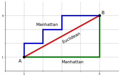
Euclidean distance: 0.527046
Manhattan distance: 1.000000
Discussion points
What does a cosine similarity of 0.5 mean?
A cosine similarity of 0.5 means the documents are moderately similar. The angle between their vectors is approximately 60 degrees. This indicates some overlap in word usage patterns but not complete similarity.
Why might cosine similarity be better than Euclidean distance for text documents?
Scale invariance: Cosine similarity focuses on the direction of vectors, not their magnitude, so document length doesn’t affect the comparison.
Normalization: It naturally handles documents of different lengths. Word frequency interpretation: It measures the relative proportion of words, which is more meaningful for text analysis than absolute differences.
Range: Cosine similarity ranges from -1 to 1, with 1 being identical, making it more interpretable for similarity measures.
Bit vectors and Sets
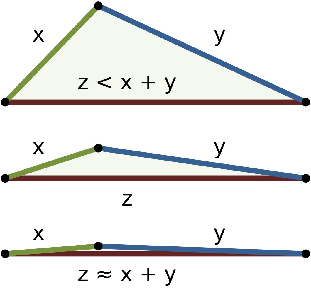
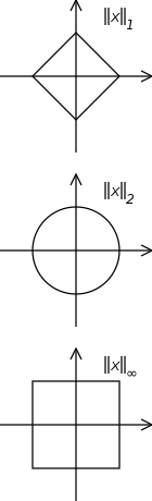
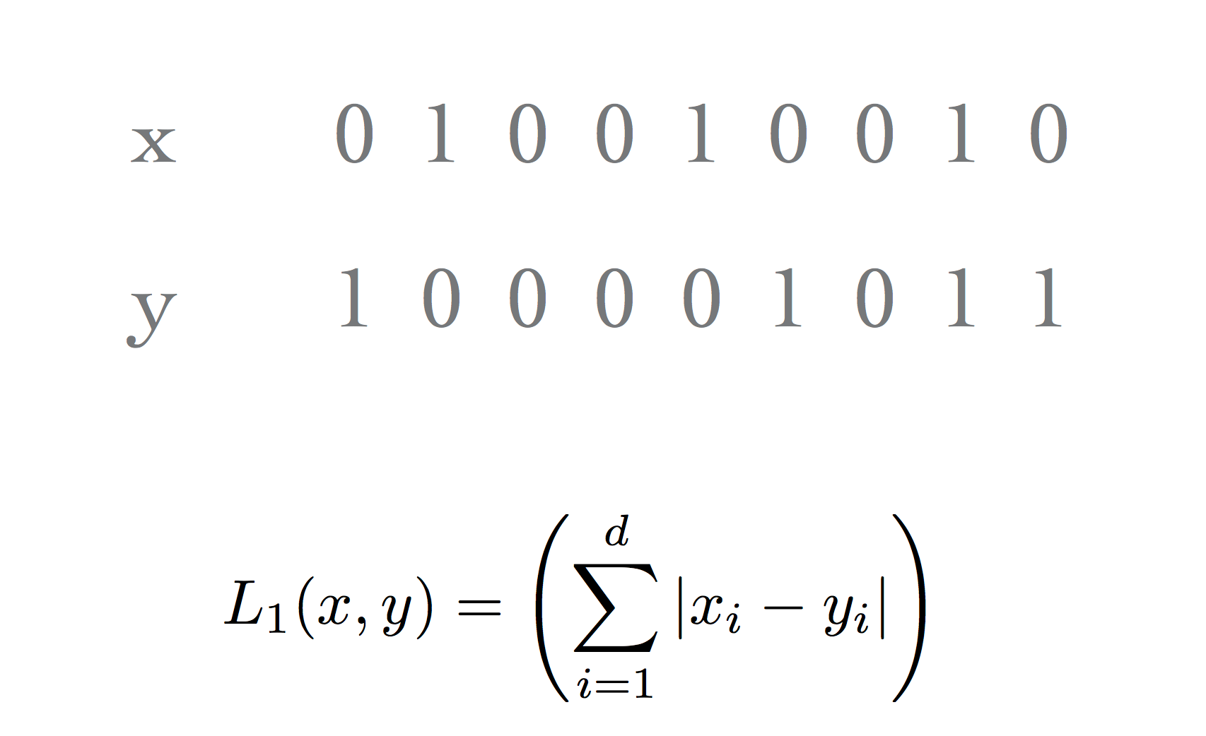
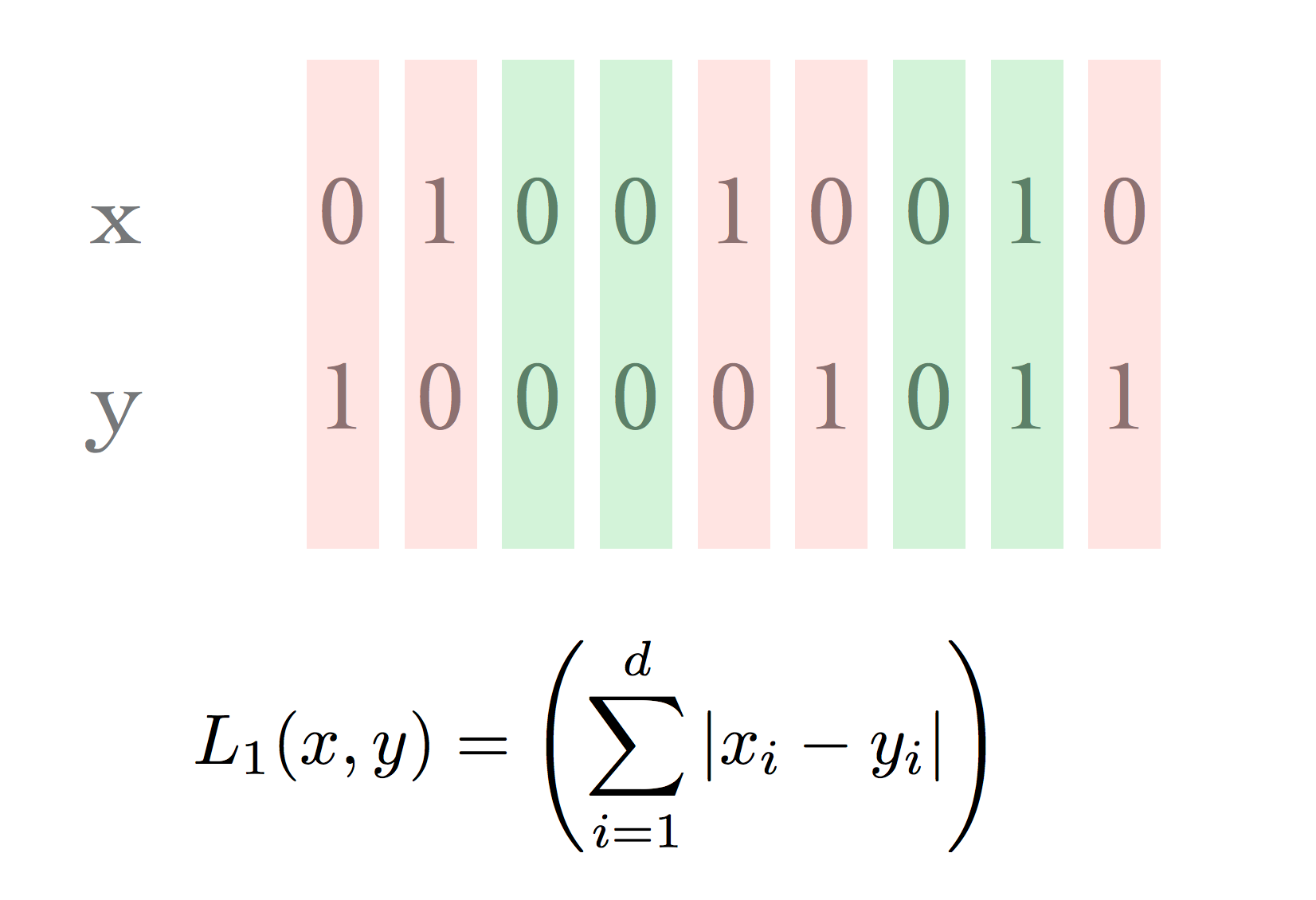
When working with bit vectors, the \(\ell_1\) metric is commonly used and is called the Hamming distance.
This has a natural interpretation: “how well do the two vectors match?”
Or: “What is the smallest number of bit flips that will convert one vector into the other?”
In other cases, the Hamming distance is not a very appropriate metric.
Consider the case in which the bit vector is being used to represent a set.
Definition: A set is an unordered collection of distinct elements.
In that case, Hamming distance measures the size of the set difference.
For example, consider two documents. We will use bit vectors to represent the sets of words in each document.
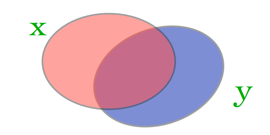
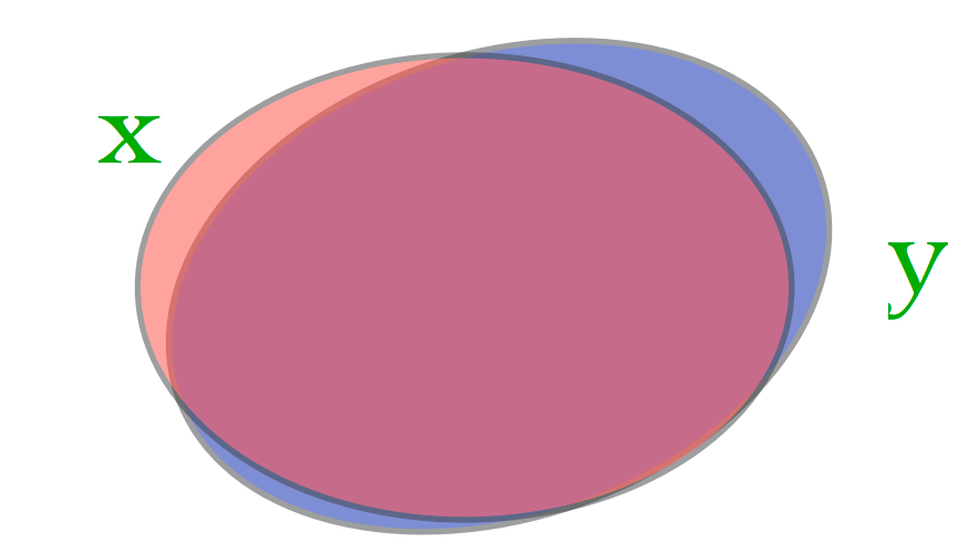
Case 1: both documents are large, almost identical, but differ in 10 words.
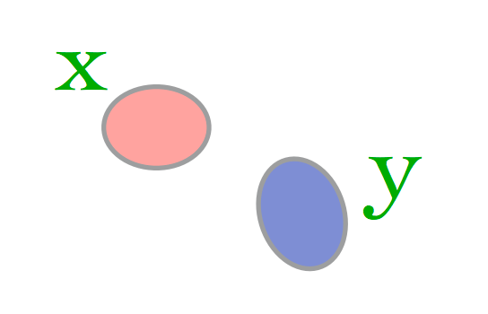
Case 2: both documents are small, disjoint, have 5 words each.
What is the Hamming distance for each case?
\(L_1(\text{Case 1}) = 10\) and \(L_1(\text{Case 2}) = 5\). Is case 1 really more different than case 2?
What matters is not just the size of the set difference, but the size of the normalized intersection.
This leads to the Jaccard similarity or Intersection over Union (IoU):
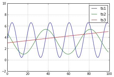
In general, there may be different aspects of a time series that are important in different settings.
The first step therefore is to ask yourself “what is important about time series in my application?”
This is an example of feature engineering.
Feature engineering is the art of computing some derived measure from your data object that makes the important properties usable in a subsequent step.
A reasonable approach is to
extract the relevant features,
use a simple method (e.g., a norm) to define similarity over those features.
In the case above, one might think of using
Fourier coefficients (to capture periodicity),
histograms,
or something else!
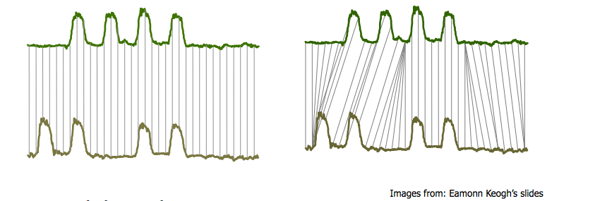
Dynamic Time Warping
One case that arises often is something like the following: “bump hunting”
Both time series have the same key characteristics: four bumps.
But a one-to-one match (ala Euclidean distance) will not detect the similarity.
(Be sure to think about why Euclidean distance will fail here.)
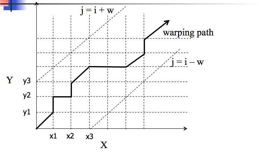
A solution to this is called dynamic time warping.
The basic idea is to allow stretching or compressing of signals along the time dimension.