Neural Networks – From Theory to Practice

Introduction

Code

import numpy as np
import matplotlib.pyplot as plt
import pandas as pd
import seaborn as sns
from IPython.display import Image, HTML
import warnings
warnings.filterwarnings('ignore')

%matplotlib inline

In this lecture, we’ll build an understanding of neural networks, starting from the foundations and moving to practical implementation using scikit-learn.

We’ll cover:

How neural networks extend linear and logistic regression
The Multi-Layer Perceptron (MLP) architecture
Gradient descent and optimization
Practical implementation with scikit-learn’s MLPClassifier and MLPRegressor

Effectiveness of Neural Networks

Applications Across Domains

From Regression to Neural Networks

Linear Regression Revisited

Recall linear regression predicts a continuous output:

\[ \hat{y} = \beta_0 + \beta_1 x_1 + \beta_2 x_2 + \cdots + \beta_p x_p = \mathbf{x}^T\boldsymbol{\beta} \]

Or in matrix form for multiple samples:

\[ \hat{\mathbf{y}} = \mathbf{X}\boldsymbol{\beta} \]

Question: What’s the main limitation of linear regression?

Answer: It can only model linear relationships between inputs and outputs!

Logistic Regression

Adds Non-linearity
For binary classification, logistic regression applies a sigmoid function:

\[ P(y=1|\mathbf{x}) = \sigma(\mathbf{x}^T\boldsymbol{\beta}) = \frac{1}{1 + e^{-\mathbf{x}^T\boldsymbol{\beta}}} \]

Logistic Regression, cont.

The sigmoid function introduces non-linearity:

The Key Insight

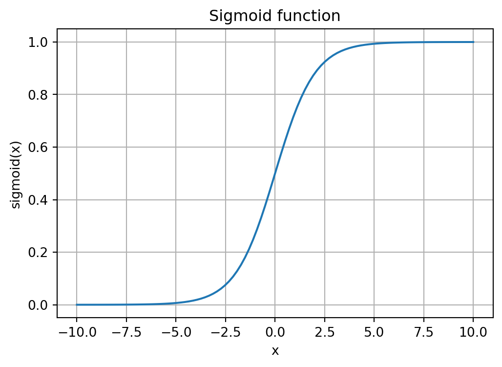
A single neuron with a sigmoid activation is essentially logistic regression!

Neural networks extend this by:

Multiple neurons in parallel (learning different features)
- Universal Approximation Theorem guarantees that a network with a single hidden layer can approximate any continuous function to any desired accuracy.
Multiple layers in sequence (learning hierarchical representations)
- Representational capacity is more efficiient
Various activation functions (ReLU, tanh, etc.)
- Required to not collapse to a single linear transformation

This allows neural networks to learn complex, non-linear decision boundaries.

Artificial Neurons

The Artificial Neuron

An artificial neuron is loosely modeled on biological neurons:

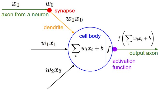
From cs231n

Neuron Components

A neuron performs the following operation:

\[ \text{output} = f\left(\sum_{i=1}^n w_i x_i + b\right) \]

Where:

$x_i$ are the inputs
$w_i$ are the weights (parameters to learn)
$b$ is the bias (another parameter)
$f$ is the activation function (introduces non-linearity)

Activation Functions

ReLU (Rectified Linear Unit) - most popular today: \[ \text{ReLU}(x) = \max(0, x) \]

Why activation functions?

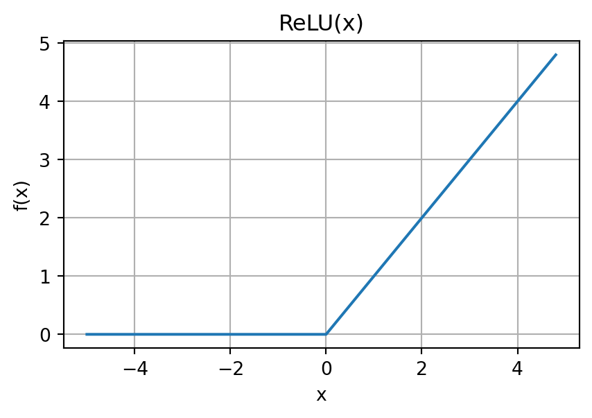
Answer: Without non-linearity, multiple layers collapse to a single linear transformation!

Multi-Layer Perceptron (MLP)

MLP Architecture

A Multi-Layer Perceptron stacks multiple layers of neurons:

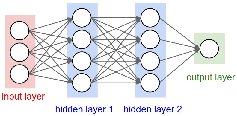
From cs231n

Input layer: Raw features
Hidden layers: Learn intermediate representations
Output layer: Final prediction

Matrix Formulation

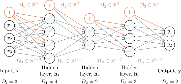
Key property: Every neuron in layer $i$ connects to every neuron in layer $i+1$.

This is also called a Fully Connected Network (FCN) or Dense Network.

MLP Mathematical Formulation

For a network with $K$ hidden layers:

\[ \begin{aligned} \mathbf{h}_1 &= f(\boldsymbol{\beta}_0 + \boldsymbol{\Omega}_0 \mathbf{x}) \\ \mathbf{h}_2 &= f(\boldsymbol{\beta}_1 + \boldsymbol{\Omega}_1 \mathbf{h}_1) \\ &\vdots \\ \mathbf{h}_K &= f(\boldsymbol{\beta}_{K-1} + \boldsymbol{\Omega}_{K-1} \mathbf{h}_{K-1}) \\ \mathbf{\hat{y}} &= \boldsymbol{\beta}_K + \boldsymbol{\Omega}_K \mathbf{h}_K \end{aligned} \]

Where:

$\mathbf{h}_k$ = hidden layer activations
$\boldsymbol{\Omega}_k$ = weight matrices
$\boldsymbol{\beta}_k$ = bias vectors
$f$ = activation function (e.g., ReLU)

Training Neural Networks

The Loss Function

Training means finding weights that minimize a loss function:

For regression (e.g., predicting house prices): \[ L = \frac{1}{N}\sum_{i=1}^N (\hat{y}_i - y_i)^2 \quad \text{(Mean Squared Error)} \]

For classification (e.g., digit recognition): \[ L = -\frac{1}{N}\sum_{i=1}^N \sum_{c=1}^C y_{ic} \log(\hat{y}_{ic}) \quad \text{(Cross-Entropy)} \]

Goal: Find parameters $\theta = \{\boldsymbol{\Omega}_k, \boldsymbol{\beta}_k\}$ that minimize $L$.

Visualizing the Loss Surface

The loss function creates a surface over the parameter space:

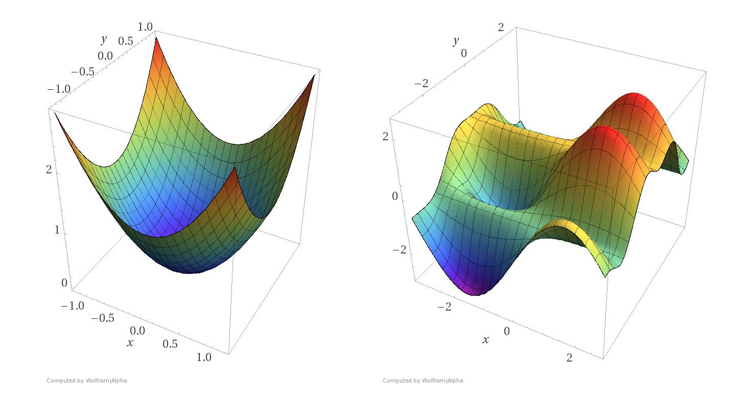
Left: Convex loss surface (e.g., linear regression)
Right: Non-convex loss surface (e.g., neural networks)

For neural networks, we can’t solve analytically—we need gradient descent!

Gradient Descent

The Gradient Descent Intuition

Imagine you’re lost in foggy mountains and want to reach the valley:

What would you do?

Look around 360 degrees
Find the direction sloping downward most steeply
Take a few steps in that direction
Repeat until the ground is level

This is gradient descent!

The Gradient

For a function $L(\mathbf{w})$ where $\mathbf{w} = (w_1, \ldots, w_n)$, the gradient is:

\[ \nabla_\mathbf{w} L(\mathbf{w}) = \begin{bmatrix} \frac{\partial L}{\partial w_1}\\ \frac{\partial L}{\partial w_2}\\ \vdots \\ \frac{\partial L}{\partial w_n} \end{bmatrix} \]

The gradient points in the direction of steepest increase
The negative gradient points toward steepest decrease

Gradient Descent Algorithm

Start with random weights $\mathbf{w}^{(0)}$, then iterate:

\[ \mathbf{w}^{(t+1)} = \mathbf{w}^{(t)} - \eta \nabla_\mathbf{w} L(\mathbf{w}^{(t)}) \]

Where:

$\eta$ is the learning rate (step size)
$\nabla_\mathbf{w} L$ is the gradient of the loss

Stop when:

Loss stops decreasing (convergence)
Maximum iterations reached

Learning Rate Matters

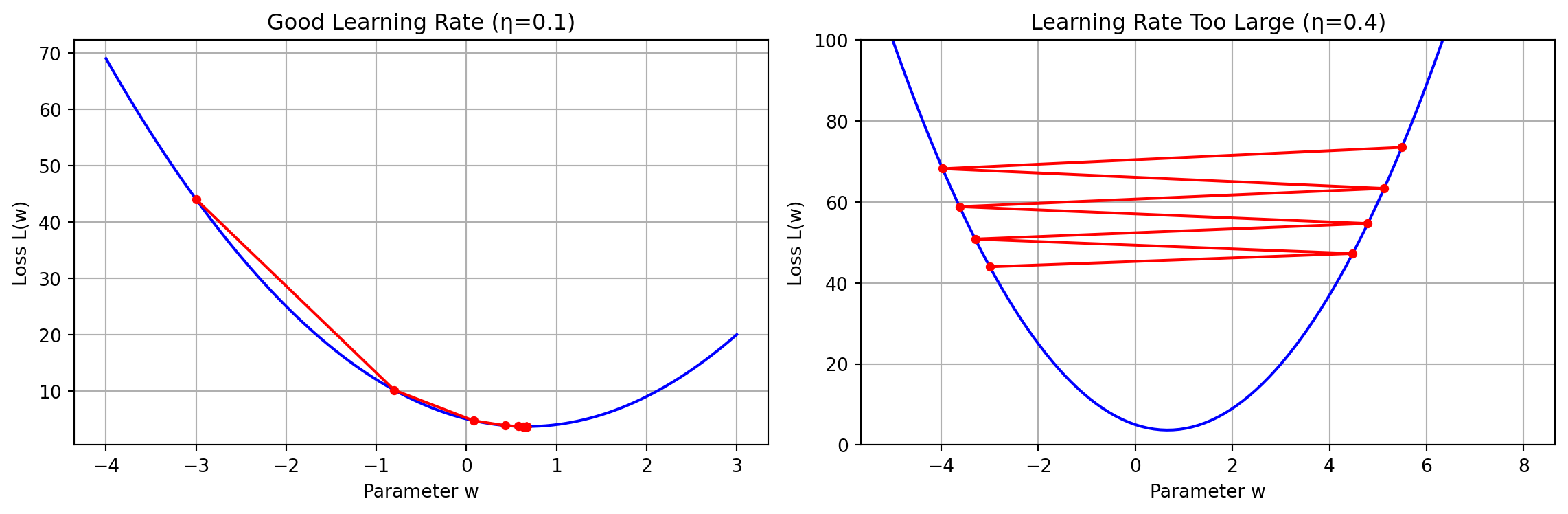
The learning rate $\eta$ is crucial:

Too small: Slow convergence

Too large: May fail to converge or even diverge!

Stochastic Gradient Descent

Full Batch vs Stochastic GD

Full Batch Gradient Descent: Compute gradient using ALL training samples:

\[ \nabla_\mathbf{w} L = \frac{1}{N}\sum_{i=1}^N \nabla_\mathbf{w} \ell_i(\mathbf{w}) \]

Problems:

Slow for large datasets (millions of samples!)
Memory intensive
Can get stuck in local minima

Stochastic Gradient Descent (SGD)

Stochastic Gradient Descent: Historically meant using ONE random sample at a time:

\[ \mathbf{w}^{(t+1)} = \mathbf{w}^{(t)} - \eta \nabla_\mathbf{w} \ell_i(\mathbf{w}^{(t)}) \]

Advantages:

Much faster per iteration
Can escape local minima (due to noise)
Enables online learning

Disadvantage:

Extremely noisy gradient estimates
May not converge exactly to minimum

Mini-Batch Gradient Descent

Mini-Batch GD: Best of both worlds—use a small batch of samples:

\[ \nabla_\mathbf{w} L \approx \frac{1}{B}\sum_{i \in \text{batch}} \nabla_\mathbf{w} \ell_i(\mathbf{w}) \]

Typical batch sizes: 32, 64, 128, 256

Advantages:

Balances speed and stability
Efficient GPU parallelization
Better gradient estimates than pure SGD

This is what most modern neural network training uses!

Visualizing Batch Strategies

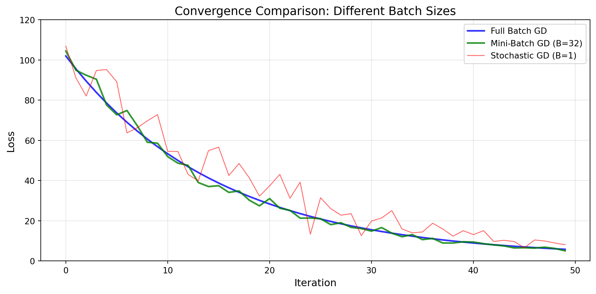
(For illustration purposes only – not a real training curve.)

Neural Networks in Scikit-Learn

MLPClassifier and MLPRegressor

Scikit-learn provides simple, high-level interfaces:

MLPClassifier: Multi-layer Perceptron classifier
MLPRegressor: Multi-layer Perceptron regressor

Key features:

Multiple hidden layers with various activation functions
Multiple solvers: 'adam', 'sgd', 'lbfgs'
Built-in regularization (L2 penalty)
Early stopping support
Easy integration with scikit-learn pipelines

Architecture Specification

Specify architecture as a tuple:

# Single hidden layer with 100 neurons
hidden_layer_sizes=(100,)

# Two hidden layers: 100 and 50 neurons
hidden_layer_sizes=(100, 50)

# Three hidden layers
hidden_layer_sizes=(128, 64, 32)

Input and output layers are automatically determined from your data!

Scikit-Learn vs PyTorch/TensorFlow

Use Scikit-Learn for:

Small to medium datasets (< 100K samples)
Standard feedforward architectures
Rapid prototyping needed
Integration with scikit-learn pipelines
CPU training is sufficient

Use PT/TF for:

Large datasets (> 100K samples)
Complex architectures (CNNs, RNNs)
GPU acceleration required
Production deployment
Research and experimentation

Classification Example: MNIST

Load the MNIST Dataset

Let’s classify handwritten digits (0-9):

from sklearn.datasets import fetch_openml
from sklearn.model_selection import train_test_split

# Load MNIST data
print("Loading MNIST dataset...")
X, y = fetch_openml('mnist_784', version=1, return_X_y=True, 
                    as_frame=False, parser='auto')

# Convert labels to integers
y = y.astype(int)

# Use subset for faster demo
X, _, y, _ = train_test_split(X, y, train_size=10000, 
                               stratify=y, random_state=42)

print(f"Dataset shape: {X.shape}")
print(f"Number of classes: {len(np.unique(y))}")

Loading MNIST dataset...
Dataset shape: (10000, 784)
Number of classes: 10

Visualize the Data

Code

fig, axes = plt.subplots(2, 5, figsize=(12, 4))
for i, ax in enumerate(axes.flat):
    ax.imshow(X[i].reshape(28, 28), cmap='gray')
    ax.set_title(f'Label: {y[i]}')
    ax.axis('off')
plt.tight_layout()
plt.show()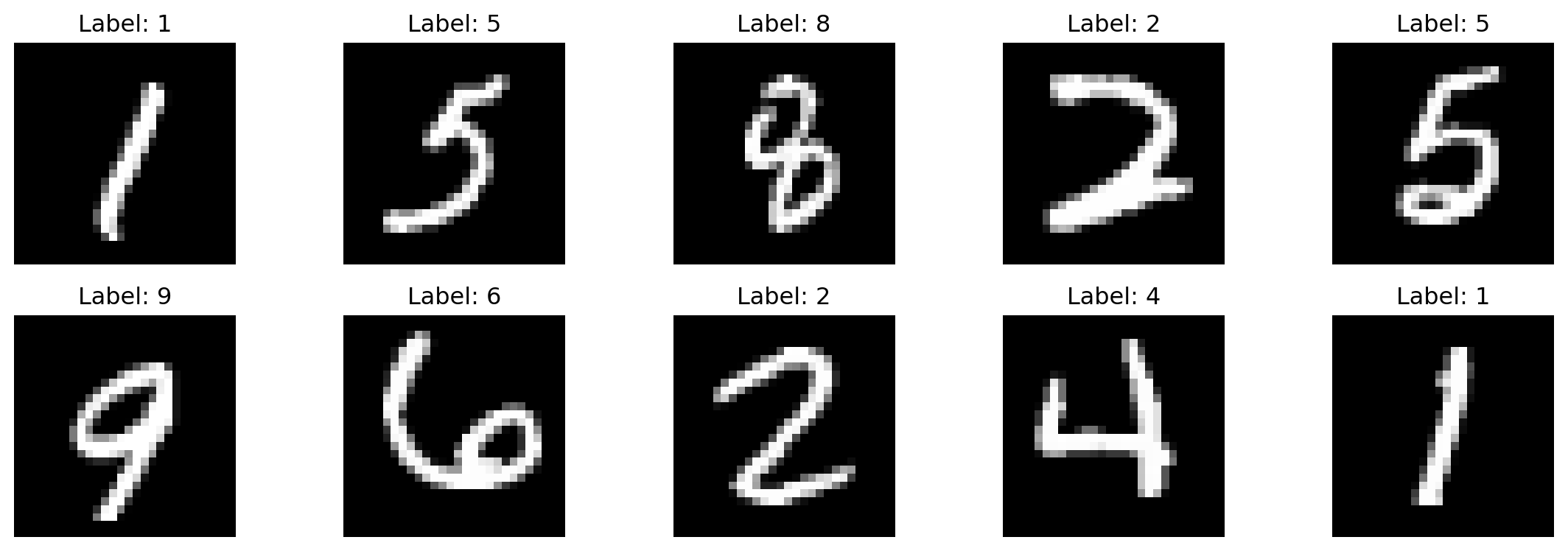

Each image is 28×28 pixels = 784 features

Prepare the Data

# Split into training and test sets
X_train, X_test, y_train, y_test = train_test_split(
    X, y, test_size=0.2, random_state=42
)

# Scale features to [0, 1]
X_train_scaled = X_train / 255.0
X_test_scaled = X_test / 255.0

print(f"Training set: {X_train.shape[0]} samples")
print(f"Test set: {X_test.shape[0]} samples")
print(f"Feature range: [{X_train_scaled.min():.2f}, {X_train_scaled.max():.2f}]")

Training set: 8000 samples
Test set: 2000 samples
Feature range: [0.00, 1.00]

Important

Always scale/normalize your features for neural networks! This helps gradient descent converge faster.

Create the MLP

from sklearn.neural_network import MLPClassifier

# Create MLP with 2 hidden layers
mlp = MLPClassifier(
    hidden_layer_sizes=(128, 64),  # Architecture
    activation='relu',              # Activation function
    solver='adam',                  # Optimizer (uses mini-batches)
    alpha=0.0001,                   # L2 regularization
    batch_size=64,                  # Mini-batch size
    learning_rate_init=0.001,       # Initial learning rate
    max_iter=20,                    # Number of epochs
    random_state=42,
    verbose=True                    # Show progress
)

Train the model

print("Training MLP...")
mlp.fit(X_train_scaled, y_train)
print(f"Training completed in {mlp.n_iter_} iterations")

Training MLP...
Iteration 1, loss = 0.71345206
Iteration 2, loss = 0.26439384
Iteration 3, loss = 0.18880844
Iteration 4, loss = 0.14070827
Iteration 5, loss = 0.10813206
Iteration 6, loss = 0.08241134
Iteration 7, loss = 0.06312883
Iteration 8, loss = 0.04742022
Iteration 9, loss = 0.03751731
Iteration 10, loss = 0.02680532
Iteration 11, loss = 0.02321482
Iteration 12, loss = 0.01516949
Iteration 13, loss = 0.01235069
Iteration 14, loss = 0.00823132
Iteration 15, loss = 0.00665425
Iteration 16, loss = 0.00515634
Iteration 17, loss = 0.00431783
Iteration 18, loss = 0.00336489
Iteration 19, loss = 0.00283319
Iteration 20, loss = 0.00253876
Training completed in 20 iterations

Training Loss Curve

Code

plt.figure(figsize=(10, 4))
plt.plot(mlp.loss_curve_)
plt.xlabel('Iteration (Epoch)')
plt.ylabel('Loss')
plt.title('Training Loss Curve')
plt.grid(True)
plt.show()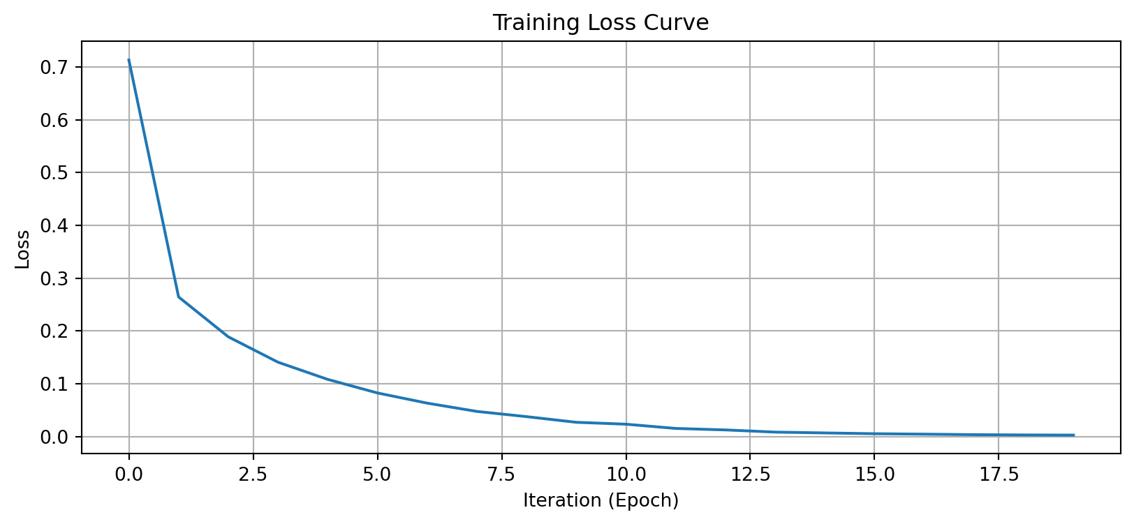

The loss decreases smoothly—our model is learning.

Evaluate Performance

Code

from sklearn.metrics import accuracy_score, classification_report

# Make predictions
y_pred = mlp.predict(X_test_scaled)

# Calculate accuracy
accuracy = accuracy_score(y_test, y_pred)
print(f"Test Accuracy: {accuracy:.4f}")

# Detailed report
print("\nClassification Report:")
print(classification_report(y_test, y_pred))

Test Accuracy: 0.9555

Classification Report:
              precision    recall  f1-score   support

           0       0.95      0.99      0.97       191
           1       0.98      1.00      0.99       226
           2       0.94      0.96      0.95       215
           3       0.95      0.93      0.94       202
           4       0.98      0.94      0.96       206
           5       0.96      0.94      0.95       168
           6       0.98      0.97      0.98       196
           7       0.93      0.96      0.95       185
           8       0.96      0.95      0.95       206
           9       0.91      0.91      0.91       205

    accuracy                           0.96      2000
   macro avg       0.96      0.96      0.96      2000
weighted avg       0.96      0.96      0.96      2000

Confusion Matrix

Code

from sklearn.metrics import confusion_matrix, ConfusionMatrixDisplay

fig, ax = plt.subplots(figsize=(8, 6))
cm = confusion_matrix(y_test, y_pred)
disp = ConfusionMatrixDisplay(confusion_matrix=cm, display_labels=mlp.classes_)
disp.plot(ax=ax, cmap='Blues', values_format='d')
plt.title('Confusion Matrix for MNIST Classification')
plt.show()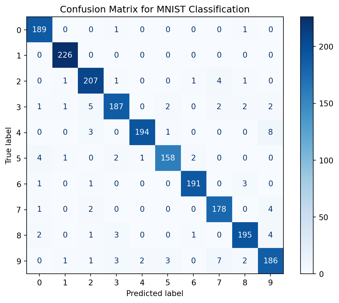

Visualize Predictions

Code

# Get prediction probabilities
y_pred_proba = mlp.predict_proba(X_test_scaled)

fig, axes = plt.subplots(2, 5, figsize=(12, 5))
for i, ax in enumerate(axes.flat):
    ax.imshow(X_test[i].reshape(28, 28), cmap='gray')
    pred_label = y_pred[i]
    true_label = y_test[i]
    confidence = y_pred_proba[i].max()
    
    color = 'green' if pred_label == true_label else 'red'
    ax.set_title(f'True: {true_label}, Pred: {pred_label}\nConf: {confidence:.2f}', 
                 color=color)
    ax.axis('off')
plt.tight_layout()
plt.show()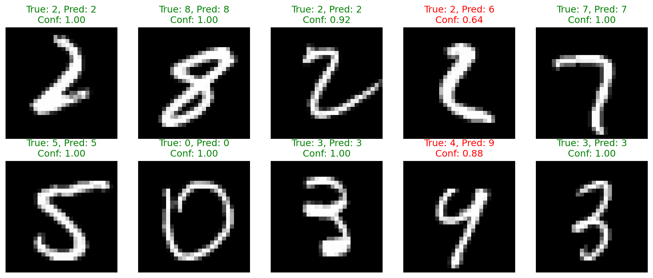

Regression Example

California Housing Dataset

Let’s predict house prices using MLP regression:

from sklearn.datasets import fetch_california_housing
from sklearn.preprocessing import StandardScaler
from sklearn.neural_network import MLPRegressor

# Load housing data
housing = fetch_california_housing()
X_housing = housing.data
y_housing = housing.target

print(f"Dataset shape: {X_housing.shape}")
print(f"Features: {housing.feature_names}")

Dataset shape: (20640, 8)
Features: ['MedInc', 'HouseAge', 'AveRooms', 'AveBedrms', 'Population', 'AveOccup', 'Latitude', 'Longitude']

Target: Median house value (in $100,000s)

Prepare Data and Define Model

# Split and scale
X_train_h, X_test_h, y_train_h, y_test_h = train_test_split(
    X_housing, y_housing, test_size=0.2, random_state=42
)

scaler = StandardScaler()
X_train_h_scaled = scaler.fit_transform(X_train_h)
X_test_h_scaled = scaler.transform(X_test_h)

# Train MLP Regressor with early stopping
mlp_reg = MLPRegressor(
    hidden_layer_sizes=(100, 50),
    activation='relu',
    solver='adam',
    alpha=0.001,
    batch_size=32,
    max_iter=100,
    early_stopping=True,
    validation_fraction=0.1,
    n_iter_no_change=10,
    random_state=42,
    verbose=False
)

Train the model

print("Training MLP Regressor...")
mlp_reg.fit(X_train_h_scaled, y_train_h)
print(f"Training stopped at iteration: {mlp_reg.n_iter_}")

Training MLP Regressor...
Training stopped at iteration: 76

Training Loss Curve

Code

plt.figure(figsize=(10, 4))
plt.plot(mlp_reg.loss_curve_)
plt.xlabel('Iteration (Epoch)')
plt.ylabel('Loss')
plt.title('Training Loss Curve')
plt.grid(True)
plt.show()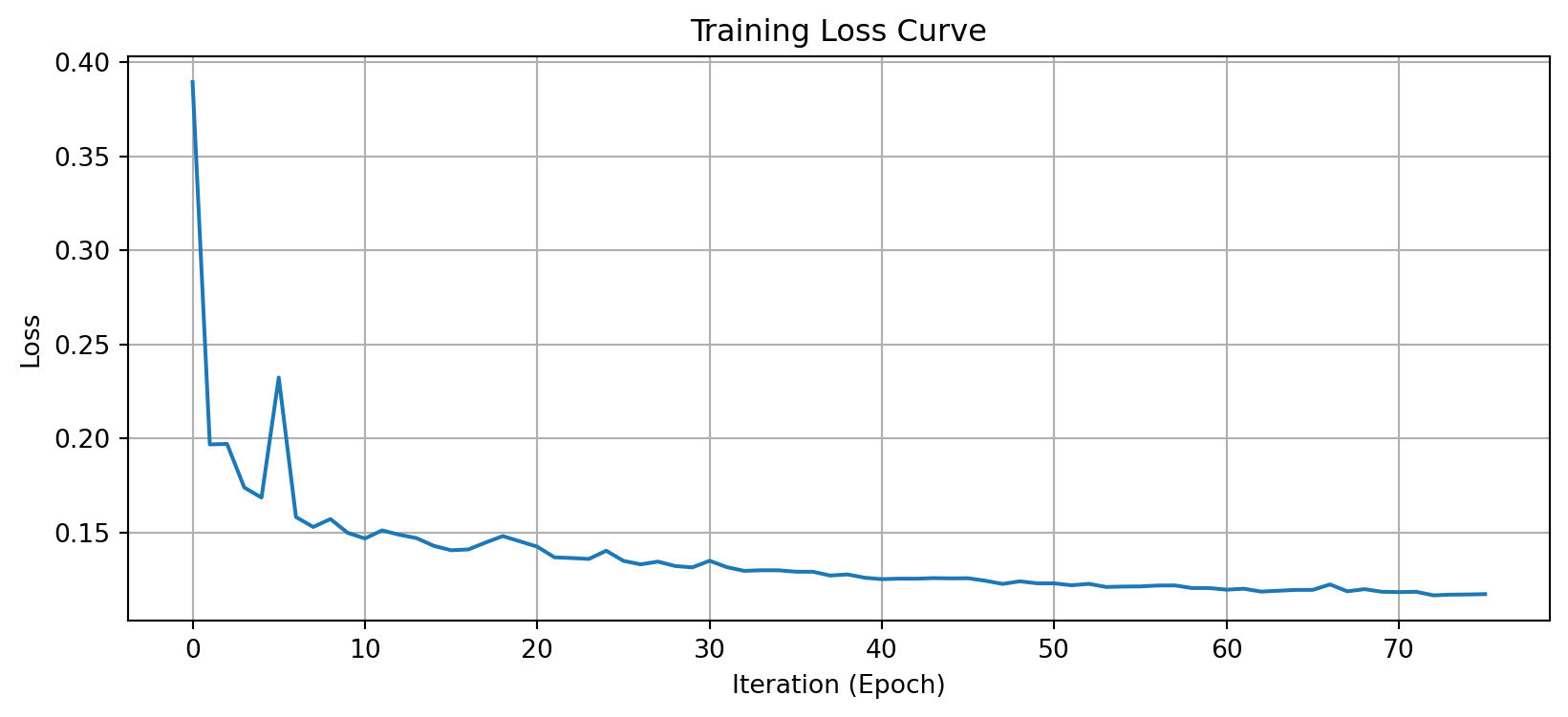

Evaluate Regression Model

from sklearn.metrics import mean_squared_error, r2_score, mean_absolute_error

# Make predictions
y_pred_h = mlp_reg.predict(X_test_h_scaled)

# Calculate metrics
mse = mean_squared_error(y_test_h, y_pred_h)
rmse = np.sqrt(mse)
mae = mean_absolute_error(y_test_h, y_pred_h)
r2 = r2_score(y_test_h, y_pred_h)

print(f"Root Mean Squared Error: {rmse:.4f}")
print(f"Mean Absolute Error: {mae:.4f}")
print(f"R² Score: {r2:.4f}")

Root Mean Squared Error: 0.5138
Mean Absolute Error: 0.3460
R² Score: 0.7986

An $R^2$ of ~0.8 means our model explains 80% of the variance in house prices!

Predictions vs Actual

Code

fig, axes = plt.subplots(1, 2, figsize=(10, 5))

# Scatter plot
axes[0].scatter(y_test_h, y_pred_h, alpha=0.5)
axes[0].plot([y_test_h.min(), y_test_h.max()], 
             [y_test_h.min(), y_test_h.max()], 'r--', lw=2)
axes[0].set_xlabel('Actual Values')
axes[0].set_ylabel('Predicted Values')
axes[0].set_title('Predicted vs Actual House Prices')
axes[0].grid(True)

# Residual plot
residuals = y_test_h - y_pred_h
axes[1].scatter(y_pred_h, residuals, alpha=0.5)
axes[1].axhline(y=0, color='r', linestyle='--', lw=2)
axes[1].set_xlabel('Predicted Values')
axes[1].set_ylabel('Residuals')
axes[1].set_title('Residual Plot')
axes[1].grid(True)

plt.tight_layout()
plt.show()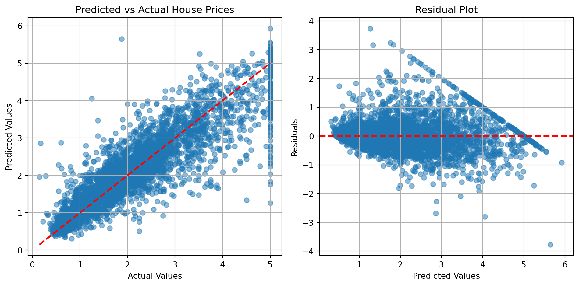

Hyperparameter Tuning

Grid Search for Optimal Architecture

scikit-learn provides GridSearchCV for hyperparameter tuning:

Create a model without certain hyperparameters.

# Create MLP
mlp_grid = MLPClassifier(
    max_iter=20,
    random_state=42,
    early_stopping=True,
    validation_fraction=0.1,
    n_iter_no_change=5,
    verbose=False
)

# Use subset for faster demo
X_grid = X_train_scaled[:1500]
y_grid = y_train[:1500]

Grid Search, cont.

Define the parameter grid and run the grid search.

from sklearn.model_selection import GridSearchCV

# Define parameter grid
param_grid = {
    'hidden_layer_sizes': [(50,), (100,), (50, 50)],
    'activation': ['relu'],
    'alpha': [0.0001, 0.001]
}

print("Running Grid Search...")
grid_search = GridSearchCV(mlp_grid, param_grid, cv=3, n_jobs=2, verbose=0)
grid_search.fit(X_grid, y_grid)

print(f"\nBest parameters: {grid_search.best_params_}")
print(f"Best CV score: {grid_search.best_score_:.4f}")

Running Grid Search...


Best parameters: {'activation': 'relu', 'alpha': 0.001, 'hidden_layer_sizes': (50,)}
Best CV score: 0.8740

Grid Search Results

Code

results_df = pd.DataFrame(grid_search.cv_results_)


n_configs = min(10, len(results_df))
top_results = results_df.nlargest(n_configs, 'mean_test_score')

# plt.figure(figsize=(10, 5))
# plt.barh(range(len(top_results)), top_results['mean_test_score'])
# plt.yticks(range(len(top_results)), 
#            [f"Config {i+1}" for i in range(len(top_results))])
# plt.xlabel('Mean CV Score')
# plt.title('Top Hyperparameter Configurations')
# plt.grid(True, axis='x')
# plt.tight_layout()
# plt.show()

print("\nTop configurations:")
for idx, row in top_results.iterrows():
    print(f"\nConfiguration {idx + 1}:")
    for key, value in row['params'].items():
        print(f"  {key}: {value}")

print("\nMean CV Score:")
print(top_results[['mean_test_score', 'std_test_score']].head())


Top configurations:

Configuration 4:
  activation: relu
  alpha: 0.001
  hidden_layer_sizes: (50,)

Configuration 1:
  activation: relu
  alpha: 0.0001
  hidden_layer_sizes: (50,)

Configuration 2:
  activation: relu
  alpha: 0.0001
  hidden_layer_sizes: (100,)

Configuration 5:
  activation: relu
  alpha: 0.001
  hidden_layer_sizes: (100,)

Configuration 6:
  activation: relu
  alpha: 0.001
  hidden_layer_sizes: (50, 50)

Configuration 3:
  activation: relu
  alpha: 0.0001
  hidden_layer_sizes: (50, 50)

Mean CV Score:
   mean_test_score  std_test_score
3         0.874000        0.007483
0         0.872000        0.008165
1         0.870667        0.016357
4         0.869333        0.015861
5         0.869333        0.010625

Best Practices

Data Preprocessing

Always preprocess your data!

Scale features: Use StandardScaler or normalize to [0, 1]
Handle missing values: Impute or remove
Encode categorical variables: One-hot encoding
Use pipelines: Ensures consistent preprocessing

from sklearn.pipeline import Pipeline

pipeline = Pipeline([
    ('scaler', StandardScaler()),
    ('mlp', MLPClassifier(hidden_layer_sizes=(100,)))
])

pipeline.fit(X_train, y_train)

Architecture Selection

Rules of thumb for architecture:

Start simple: Try single hidden layer first
Layer sizes: Between input and output dimensions
Depth vs width:
- More layers → learn complex patterns
- But risk overfitting on small data
Typical architectures:
- Small data: (100,) or (50, 50)
- Medium data: (100, 50) or (128, 64, 32)
- Large data: Consider PyTorch

Preventing Overfitting

Three key techniques:

1. Regularization: Add L2 penalty (alpha parameter)

mlp = MLPClassifier(alpha=0.01)  # Stronger regularization

2. Early Stopping: Stop when validation performance plateaus

mlp = MLPClassifier(early_stopping=True, 
                    validation_fraction=0.2,
                    n_iter_no_change=10)

3. Cross-Validation: Get robust performance estimates

from sklearn.model_selection import cross_val_score
scores = cross_val_score(mlp, X_train, y_train, cv=5)

Solver Selection

Different solvers for different scenarios:

Solver	Best For	Notes
`'adam'`	Most cases	Good default, adaptive learning rate
`'sgd'`	Large datasets	Classic mini-batch SGD
`'lbfgs'`	Small datasets	Faster for small data, more memory

Code

# Compare solvers
solvers = ['adam', 'sgd', 'lbfgs']
results = {}

for solver in solvers:
    mlp = MLPClassifier(
        hidden_layer_sizes=(50,),
        solver=solver,
        max_iter=50,
        random_state=42,
        verbose=False
    )
    mlp.fit(X_train_scaled[:2000], y_train[:2000])
    score = mlp.score(X_test_scaled, y_test)
    results[solver] = score
    print(f"{solver:10s}: {score:.4f}")

adam      : 0.9000
sgd       : 0.8330
lbfgs     : 0.8800

Common Issues

Convergence Warnings

If you see ConvergenceWarning:

Increase max_iter
Decrease learning_rate_init
Enable early_stopping=True
Check if data is properly scaled

Poor Performance

If accuracy is low:

Is data scaled/normalized?
Is architecture appropriate?
Is learning rate too high/low?
Do you need more iterations?
Is regularization too strong?

Summary

Theory:

Neural networks extend linear/logistic regression with multiple layers and non-linearity
MLPs learn hierarchical representations through hidden layers
Gradient descent optimizes the loss function
Mini-batch GD balances speed and stability

Practice:

Scikit-learn’s MLPClassifier and MLPRegressor for easy implementation
Always preprocess/scale your data
Use early stopping and regularization to prevent overfitting
Grid search helps find optimal hyperparameters

To Dig Deeper

Other modules in the course notes:

Additional resources:

Understanding Deep Learning, Simon J.D. Prince, MIT Press, 2023
DS542, Deep Learning for Data Science