GMM Appendix B: Covariance Matrix Structure in Multivariate Gaussians

The Multivariate Gaussian¹

For a \(d\)-dimensional Gaussian distribution:

\[ p(\mathbf{x} \mid \boldsymbol{\mu}, \boldsymbol{\Sigma}) = \frac{1}{(2\pi)^{d/2}|\boldsymbol{\Sigma}|^{1/2}} \exp\left(-\frac{1}{2}(\mathbf{x}-\boldsymbol{\mu})^T\boldsymbol{\Sigma}^{-1}(\mathbf{x}-\boldsymbol{\mu})\right) \]

The covariance matrix \(\boldsymbol{\Sigma}\) is a \(d \times d\) positive definite matrix that completely determines the shape, orientation, and spread of the distribution.

---

Different Forms of Covariance Matrices

1. Full Covariance Matrix (Unrestricted)

\[ \boldsymbol{\Sigma}_{\text{full}} = \begin{pmatrix} \sigma_1^2 & \sigma_{12} & \cdots & \sigma_{1d} \\ \sigma_{21} & \sigma_2^2 & \cdots & \sigma_{2d} \\ \vdots & \vdots & \ddots & \vdots \\ \sigma_{d1} & \sigma_{d2} & \cdots & \sigma_d^2 \end{pmatrix} \]

Properties:

• Symmetric: \(\sigma_{ij} = \sigma_{ji}\)
• Number of free parameters: \(\frac{d(d+1)}{2}\)
• Can represent any orientation and shape

Geometric Interpretation:

• Ellipsoids can be oriented in any direction
• Each dimension can have different variance
• Dimensions can be correlated (non-axis-aligned)

Example (2D): \[ \boldsymbol{\Sigma} = \begin{pmatrix} 2 & 1 \\ 1 & 3 \end{pmatrix} \]

Creates an ellipse tilted at an angle, not aligned with coordinate axes.

import numpy as np
import matplotlib.pyplot as plt
from scipy.stats import multivariate_normal

# Full covariance matrix
mean_full = [0, 0]
cov_full = [[2, 1],
            [1, 3]]

# Create grid
x = np.linspace(-5, 5, 100)
y = np.linspace(-5, 5, 100)
X, Y = np.meshgrid(x, y)
pos = np.dstack((X, Y))

# Calculate PDF
rv_full = multivariate_normal(mean_full, cov_full)
Z_full = rv_full.pdf(pos)

# Plot
plt.figure(figsize=(8, 8))
plt.contour(X, Y, Z_full, levels=10, cmap='viridis')
plt.title('Full Covariance: Tilted Ellipse', fontsize=14)
plt.xlabel('x₁')
plt.ylabel('x₂')
plt.axis('equal')
plt.grid(True, alpha=0.3)
plt.colorbar(label='Probability Density')
plt.show()

Usage in GMMs:

• Most flexible, can fit complex cluster shapes
• Most expensive: requires \(O(d^2)\) parameters per component
• Can overfit with limited data

---

2. Diagonal Covariance Matrix

\[ \boldsymbol{\Sigma}_{\text{diag}} = \begin{pmatrix} \sigma_1^2 & 0 & \cdots & 0 \\ 0 & \sigma_2^2 & \cdots & 0 \\ \vdots & \vdots & \ddots & \vdots \\ 0 & 0 & \cdots & \sigma_d^2 \end{pmatrix} \]

Properties:

• All off-diagonal elements are zero: \(\sigma_{ij} = 0\) for \(i \neq j\)
• Number of free parameters: \(d\)
• Dimensions are independent (uncorrelated)

Geometric Interpretation:

• Ellipsoids are axis-aligned (principal axes parallel to coordinate axes)
• Each dimension can have different spread
• No rotation or tilt

Example (2D): \[ \boldsymbol{\Sigma} = \begin{pmatrix} 2 & 0 \\ 0 & 4 \end{pmatrix} \]

Creates an axis-aligned ellipse (wider in the \(y\)-direction).

# Diagonal covariance matrix
mean_diag = [0, 0]
cov_diag = [[2, 0],
            [0, 4]]

# Calculate PDF
rv_diag = multivariate_normal(mean_diag, cov_diag)
Z_diag = rv_diag.pdf(pos)

# Plot
plt.figure(figsize=(8, 8))
plt.contour(X, Y, Z_diag, levels=10, cmap='viridis')
plt.title('Diagonal Covariance: Axis-Aligned Ellipse', fontsize=14)
plt.xlabel('x₁')
plt.ylabel('x₂')
plt.axis('equal')
plt.grid(True, alpha=0.3)
plt.colorbar(label='Probability Density')
plt.show()

Usage in GMMs:

• Good balance between flexibility and computational efficiency
• Assumes features are independent within each cluster
• Commonly used default in practice (e.g., scikit-learn’s default)
• Much faster than full covariance

---

3. Spherical (Isotropic) Covariance Matrix

\[ \boldsymbol{\Sigma}_{\text{spherical}} = \sigma^2 \mathbf{I} = \begin{pmatrix} \sigma^2 & 0 & \cdots & 0 \\ 0 & \sigma^2 & \cdots & 0 \\ \vdots & \vdots & \ddots & \vdots \\ 0 & 0 & \cdots & \sigma^2 \end{pmatrix} \]

Properties:

• All dimensions have the same variance: \(\sigma_i^2 = \sigma^2\) for all \(i\)
• Number of free parameters: \(1\)
• Special case of diagonal covariance

Geometric Interpretation: - Contours are hyperspheres (circles in 2D, spheres in 3D) - Equal spread in all directions - No preferred direction

Example (2D): \[ \boldsymbol{\Sigma} = \begin{pmatrix} 2 & 0 \\ 0 & 2 \end{pmatrix} \]

Creates a perfect circle centered at the mean.

# Spherical covariance matrix
mean_spher = [0, 0]
cov_spher = [[2, 0],
             [0, 2]]

# Calculate PDF
rv_spher = multivariate_normal(mean_spher, cov_spher)
Z_spher = rv_spher.pdf(pos)

# Plot
plt.figure(figsize=(8, 8))
plt.contour(X, Y, Z_spher, levels=10, cmap='viridis')
plt.title('Spherical Covariance: Perfect Circle', fontsize=14)
plt.xlabel('x₁')
plt.ylabel('x₂')
plt.axis('equal')
plt.grid(True, alpha=0.3)
plt.colorbar(label='Probability Density')
plt.show()

Usage in GMMs:

• Most restrictive, assumes all dimensions have equal variance
• Very efficient: only 1 parameter per component
• Suitable when features are on similar scales and have similar variability
• Often too restrictive for real data

---

4. Tied (Shared) Covariance Matrix

All mixture components share the same covariance matrix:

\[\boldsymbol{\Sigma}_1 = \boldsymbol{\Sigma}_2 = \cdots = \boldsymbol{\Sigma}_K = \boldsymbol{\Sigma}_{\text{shared}}\]

Properties:

• Can be full, diagonal, or spherical
• Number of parameters doesn’t scale with \(K\)
• All clusters have the same shape and orientation

Geometric Interpretation:

• All ellipsoids have the same shape, size, and orientation
• Only the centers (means) differ between components
• This is equivalent to Linear Discriminant Analysis (LDA) for classification

Usage in GMMs:

• Reduces overfitting when clusters have similar shapes
• Much more parameter-efficient
• Appropriate when clusters differ mainly in location, not shape

---

Visual Comparison of All Types

# Create a 2x2 subplot comparing all covariance types
fig, axes = plt.subplots(2, 2, figsize=(8, 8))

# Full covariance
ax1 = axes[0, 0]
ax1.contour(X, Y, Z_full, levels=10, cmap='viridis')
ax1.set_title('Full Covariance\n(Tilted Ellipse)', fontsize=12, fontweight='bold')
ax1.set_xlabel('x₁')
ax1.set_ylabel('x₂')
ax1.axis('equal')
ax1.grid(True, alpha=0.3)

# Diagonal covariance
ax2 = axes[0, 1]
ax2.contour(X, Y, Z_diag, levels=10, cmap='viridis')
ax2.set_title('Diagonal Covariance\n(Axis-Aligned Ellipse)', fontsize=12, fontweight='bold')
ax2.set_xlabel('x₁')
ax2.set_ylabel('x₂')
ax2.axis('equal')
ax2.grid(True, alpha=0.3)

# Spherical covariance
ax3 = axes[1, 0]
ax3.contour(X, Y, Z_spher, levels=10, cmap='viridis')
ax3.set_title('Spherical Covariance\n(Perfect Circle)', fontsize=12, fontweight='bold')
ax3.set_xlabel('x₁')
ax3.set_ylabel('x₂')
ax3.axis('equal')
ax3.grid(True, alpha=0.3)

# Tied covariance (example with 3 components)
ax4 = axes[1, 1]
means_tied = [[-2, 0], [2, 0], [0, 2.5]]
cov_tied = [[1.5, 0.5], [0.5, 1.5]]
for mean in means_tied:
    rv_tied = multivariate_normal(mean, cov_tied)
    Z_tied = rv_tied.pdf(pos)
    ax4.contour(X, Y, Z_tied, levels=8, cmap='viridis', alpha=0.7)
ax4.set_title('Tied Covariance\n(3 Components, Same Shape)', fontsize=12, fontweight='bold')
ax4.set_xlabel('x₁')
ax4.set_ylabel('x₂')
ax4.axis('equal')
ax4.grid(True, alpha=0.3)

plt.tight_layout()
plt.show()

---

GMM Example with Different Covariance Types

from sklearn.mixture import GaussianMixture
from sklearn.datasets import make_blobs

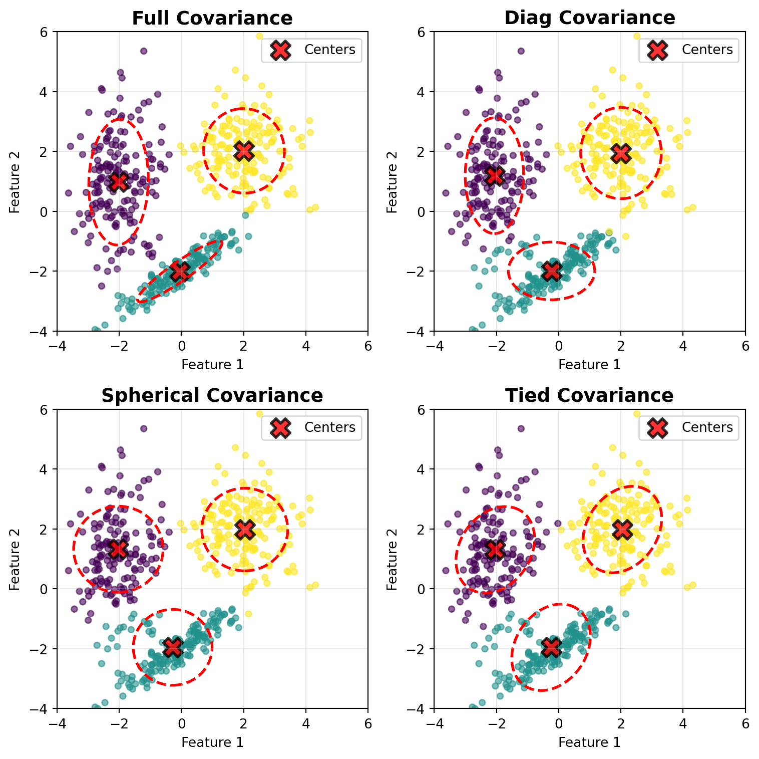
# Generate synthetic data with 3 clusters using different covariance matrices
from sklearn.datasets import make_classification
from sklearn.model_selection import train_test_split

# Create data with different covariance structures
np.random.seed(42)

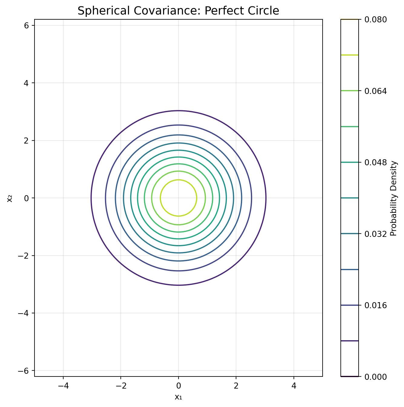
# Cluster 1: Spherical (circular)
n1 = 167
X1 = np.random.multivariate_normal([2, 2], [[1.0, 0], [0, 1.0]], n1)
y1 = np.zeros(n1)

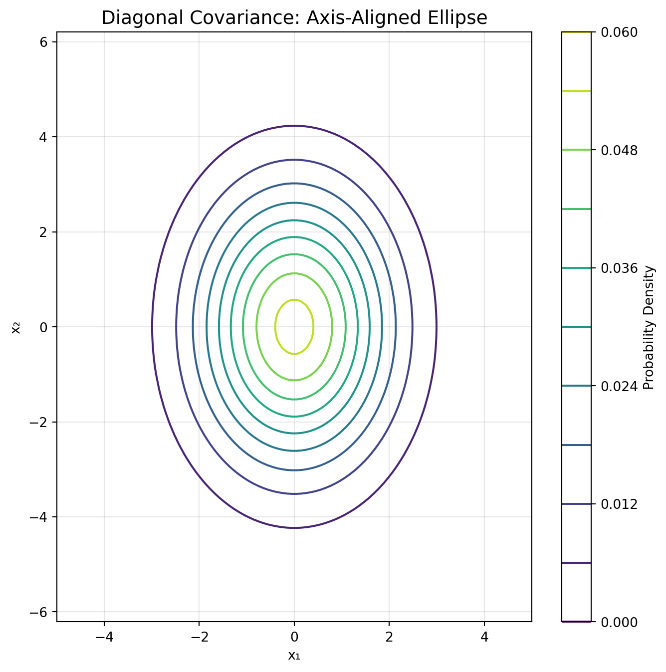
# Cluster 2: Diagonal (axis-aligned ellipse, wider in y)
n2 = 167  
X2 = np.random.multivariate_normal([-2, 1], [[0.5, 0], [0, 2.0]], n2)
y2 = np.ones(n2)

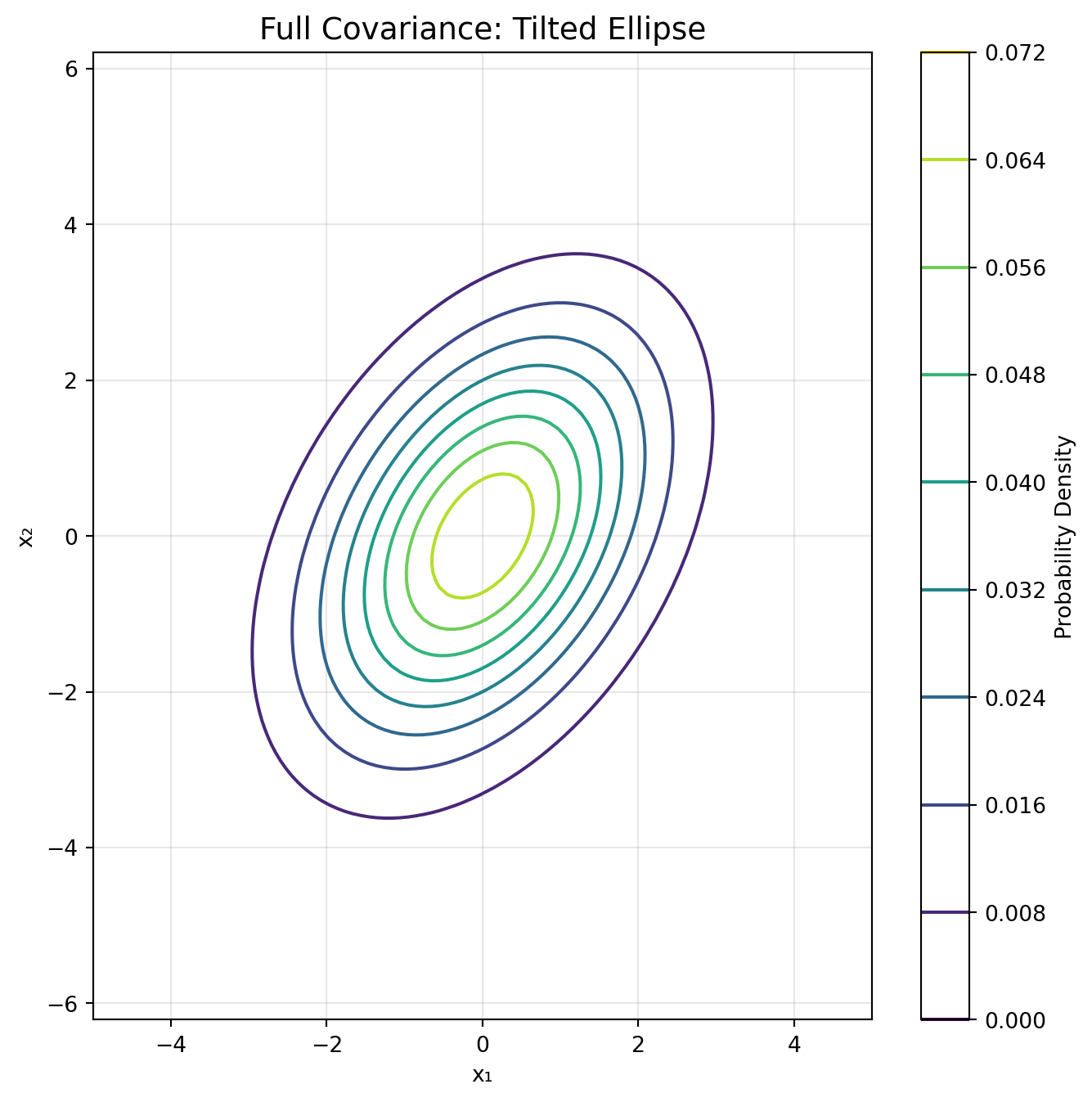
# Cluster 3: Full covariance (tilted ellipse)
n3 = 166
cov3 = np.array([[1.2, 0.8], [0.8, 0.6]])  # Positive correlation
X3 = np.random.multivariate_normal([0, -2], cov3, n3)
y3 = np.full(n3, 2)

# Combine all clusters
X = np.vstack([X1, X2, X3])
y_true = np.hstack([y1, y2, y3])

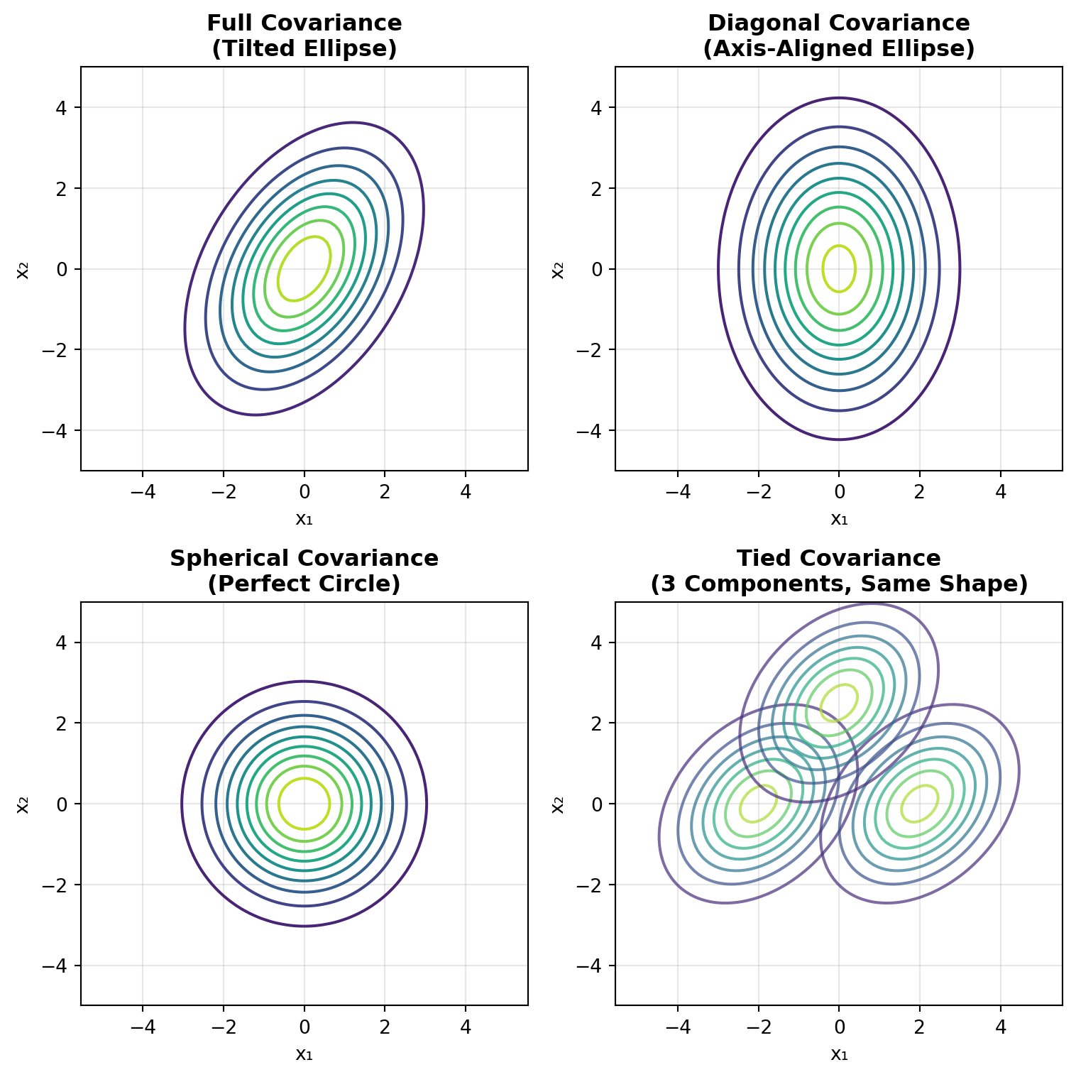
# Fit GMMs with different covariance types
covariance_types = ['full', 'diag', 'spherical', 'tied']
fig, axes = plt.subplots(2, 2, figsize=(8, 8))

for idx, (cov_type, ax) in enumerate(zip(covariance_types, axes.ravel())):
    # Fit GMM
    gmm = GaussianMixture(n_components=3, covariance_type=cov_type, random_state=42)
    gmm.fit(X)
    labels = gmm.predict(X)
    
    # Plot data points colored by cluster
    scatter = ax.scatter(X[:, 0], X[:, 1], c=labels, s=20, cmap='viridis', alpha=0.6)
    
    # Plot cluster centers
    centers = gmm.means_
    ax.scatter(centers[:, 0], centers[:, 1], c='red', s=200, alpha=0.8, 
               marker='X', edgecolors='black', linewidths=2, label='Centers')
    
    # Draw confidence ellipses for each component
    from matplotlib.patches import Ellipse
    import matplotlib.transforms as transforms
    
    for i in range(3):
        if cov_type == 'full':
            covariance = gmm.covariances_[i]
        elif cov_type == 'diag':
            covariance = np.diag(gmm.covariances_[i])
        elif cov_type == 'spherical':
            covariance = gmm.covariances_[i] * np.eye(2)
        elif cov_type == 'tied':
            covariance = gmm.covariances_
        
        # Calculate eigenvalues and eigenvectors
        v, w = np.linalg.eigh(covariance)
        v = 2.0 * np.sqrt(2.0) * np.sqrt(v)  # 95% confidence
        angle = np.degrees(np.arctan2(w[1, 0], w[0, 0]))
        
        # Draw ellipse
        ell = Ellipse(centers[i], v[0], v[1], angle=angle, 
                     edgecolor='red', facecolor='none', linewidth=2, linestyle='--')
        ax.add_patch(ell)
    
    ax.set_title(f'{cov_type.capitalize()} Covariance', fontsize=14, fontweight='bold')
    ax.set_xlabel('Feature 1')
    ax.set_ylabel('Feature 2')
    ax.set_xlim([-4, 6])
    ax.set_ylim([-4, 6])
    ax.legend()
    ax.grid(True, alpha=0.3)

plt.tight_layout()
plt.show()

# Print BIC scores for comparison
print("\nBIC Scores (lower is better):")
for cov_type in covariance_types:
    gmm = GaussianMixture(n_components=3, covariance_type=cov_type, random_state=42)
    gmm.fit(X)
    print(f"  {cov_type.capitalize()}: {gmm.bic(X):.2f}")

BIC Scores (lower is better):
  Full: 3538.70
  Diag: 3782.72
  Spherical: 3846.10
  Tied: 3815.55

---

Number of Parameters

For a GMM with \(K\) components in \(d\) dimensions:

Covariance Type	Parameters per Component	Total Covariance Parameters
Full	\(\frac{d(d+1)}{2}\)	\(K \cdot \frac{d(d+1)}{2}\)
Diagonal	\(d\)	\(K \cdot d\)
Spherical	\(1\)	\(K\)
Tied Full	\(\frac{d(d+1)}{2}\)	\(\frac{d(d+1)}{2}\)
Tied Diagonal	\(d\)	\(d\)
Tied Spherical	\(1\)	\(1\)

# Calculate number of parameters for different scenarios
def count_parameters(K, d, cov_type, tied=False):
    """Count covariance parameters in a GMM"""
    if cov_type == 'full':
        params_per_component = d * (d + 1) // 2
    elif cov_type == 'diag':
        params_per_component = d
    elif cov_type == 'spherical':
        params_per_component = 1
    
    if tied:
        return params_per_component
    else:
        return K * params_per_component

# Example: K=5 components, d=10 dimensions
K, d = 5, 10

print(f"Parameter counts for K={K} components in d={d} dimensions:\n")
print(f"  Full:           {count_parameters(K, d, 'full', tied=False)} parameters")
print(f"  Diagonal:       {count_parameters(K, d, 'diag', tied=False)} parameters")
print(f"  Spherical:      {count_parameters(K, d, 'spherical', tied=False)} parameters")
print(f"  Tied Full:      {count_parameters(K, d, 'full', tied=True)} parameters")
print(f"  Tied Diagonal:  {count_parameters(K, d, 'diag', tied=True)} parameters")
print(f"  Tied Spherical: {count_parameters(K, d, 'spherical', tied=True)} parameters")

Parameter counts for K=5 components in d=10 dimensions:

  Full:           275 parameters
  Diagonal:       50 parameters
  Spherical:      5 parameters
  Tied Full:      55 parameters
  Tied Diagonal:  10 parameters
  Tied Spherical: 1 parameters

---

Choosing the Right Covariance Structure

Use Full Covariance when:

• You have lots of data relative to dimensionality
• Clusters have different shapes and orientations
• Features are correlated within clusters
• Maximum flexibility is needed

Use Diagonal Covariance when:

• Features are approximately independent
• You want computational efficiency
• Data is moderately sized
• A good default choice for many applications

Use Spherical Covariance when:

• Features are on similar scales
• You have limited data
• Clusters are roughly circular/spherical
• Maximum computational efficiency needed

Use Tied Covariance when:

• Clusters have similar shapes but different locations
• You want to reduce overfitting
• You have limited data
• Similar to LDA assumptions

---

Footnotes

1. Courtesy of Claude.ai