Decision Tree and Random Forest Regression

Introduction

While linear and logistic regression are powerful tools, they assume specific relationships between variables (linear for continuous outcomes, logistic for binary outcomes). What if the relationship is more complex? Enter decision tree regression and random forest regression - flexible methods that can capture non-linear patterns and interactions without explicit feature engineering.

Decision Tree Regression

What is Decision Tree Regression?

The Big Picture

Imagine you’re estimating house prices.

Instead of fitting a straight line (linear regression), you ask a series of yes/no questions:

  • Is the house bigger than 2000 sq ft?
  • Does it have more than 3 bedrooms?
  • Is it in neighborhood A or B?

Each question splits your data into smaller groups, and at the end, you predict the average price of houses in each final group.

How It Works: The Mechanics

A decision tree regression model works by:

  1. Splitting the data: Find the feature and threshold that best divides your data into two groups
  2. Recursing: Repeat the process on each group
  3. Stopping: When groups are “pure enough” or meet stopping criteria
  4. Predicting: For a new data point, follow the tree down to a leaf and return the average value of training points in that leaf

Ex. 1: Simple House Price Prediction

Let’s say we have this tiny dataset:

Square Feet Bedrooms Price ($1000s)
1200 2 200
1400 2 220
1600 3 280
1800 3 300
2000 4 380
2200 4 400


The tree might look like:

           [Square Feet < 1700?]
                /          \
              Yes           No
              /              \
        [Avg: 230K]    [Bedrooms < 4?]
                           /         \
                         Yes          No
                         /             \
                   [Avg: 290K]    [Avg: 390K]

Prediction for a 1500 sq ft, 2 BR house: Follow left → predict $230K
Prediction for a 1900 sq ft, 3 BR house: Follow right → left → predict $290K

Example 2: Visualizing the Split

Consider predicting a person’s salary based on years of experience and education level.

Data points (Years_Experience, Education_Years, Salary):
(1, 12, 35K), (2, 12, 40K), (3, 16, 55K), (4, 16, 60K),
(5, 18, 70K), (6, 18, 75K), (10, 18, 90K), (12, 20, 110K)


The decision tree creates rectangular regions in the feature space:

        [Years_Experience < 4?]
             /            \
           Yes             No
           /                \
    [Edu_Years < 14?]   [Years_Exp < 8?]
       /        \           /         \
     Yes        No        Yes          No
     /          \         /             \
[Avg: 37.5K] [Avg: 57.5K] [Avg: 78.3K] [Avg: 100K]


Key Insight: Unlike linear regression which fits a single plane, decision trees partition the space into rectangles, each with its own prediction.

How Are Splits Chosen?

The algorithm minimizes residual sum of squares (RSS) at each split:

\[RSS = \sum_{i \in \text{left}} (y_i - \bar{y}_{\text{left}})^2 + \sum_{j \in \text{right}} (y_j - \bar{y}_{\text{right}})^2\]

Where \(\bar{y}_{\text{left}}\) and \(\bar{y}_{\text{right}}\) are the average values in each resulting group.


Intuition: Find the split that makes each side as “homogeneous” as possible - minimize the variance within each group.

Example 3: Temperature Prediction

Suppose we’re predicting daily high temperature based on the month:

Month Temperature (°F)
1 35
2 38
3 45
4 58
5 70
6 80
7 85
8 83
9 75
10 60
11 48
12 37

A decision tree might split like this:

            [Month < 6.5?]
               /        \
             Yes         No
             /            \
      [Month < 3.5?]  [Month < 9.5?]
         /      \         /       \
       Yes      No      Yes        No
       /         \       /          \
   [Avg: 36°] [Avg: 58°] [Avg: 81°] [Avg: 48°]


This captures the non-linear relationship (winter → spring → summer → fall) that linear regression would struggle with.

Piecewise Constant Predictions

Understanding Discretized Outputs

Critical characteristic of decision tree regression: outputs are always discretized.

When you train a tree, each leaf node stores a single prediction value (the mean of all training samples in that leaf).

No matter how many different inputs you provide, the model can only produce as many distinct values as it has leaf nodes.


Key Insight: If your tree has 10 leaf nodes, it can only produce 10 unique predictions - ever.

Ex.: Sweeping Through Input Values

Let’s see this in action with a simple example of eight values:

[10, 15, 25, 40, 60, 85, 115, 150]

and train a small decision tree with only 4 leaf nodes.

Code
import numpy as np
from sklearn.tree import DecisionTreeRegressor
import matplotlib.pyplot as plt

# Simple quadratic relationship
X_train = np.array([[1], [2], [3], [4], [5], [6], [7], [8]])
y_train = np.array([10, 15, 25, 40, 60, 85, 115, 150])  # roughly x^2

# Shallow tree with only 4 leaf nodes
tree = DecisionTreeRegressor(max_depth=2, random_state=42)
tree.fit(X_train, y_train)

# Sweep through 100 input values
X_test = np.linspace(0, 10, 100).reshape(-1, 1)
predictions = tree.predict(X_test)

print(f"Number of unique predictions: {len(np.unique(predictions))}")
print(f"Unique values: {np.unique(predictions)}")

# Output:
# Number of unique predictions: 4
# Unique values: [12.5, 32.5, 72.5, 132.5]
Number of unique predictions: 4
Unique values: [ 16.66666667  50.         100.         150.        ]

Visualizing the Step Function

When you plot predictions from a decision tree, you see a step function:

Code
plt.figure(figsize=(8, 3))

# Plot the step function
plt.plot(X_test, predictions, 'r-', linewidth=2, label='Decision Tree', drawstyle='steps-post')

# Plot training data
plt.scatter(X_train, y_train, s=100, alpha=0.6, edgecolors='black', label='Training Data')

# Plot the true function for comparison
y_true = X_test**2
# plt.plot(X_test, y_true, 'g--', alpha=0.5, linewidth=2, label='True Function (x²)')

plt.xlabel('Input (x)', fontsize=12)
plt.ylabel('Prediction (y)', fontsize=12)
plt.title('Decision Tree Creates Step Functions', fontsize=14)
plt.legend(fontsize=11)
plt.grid(alpha=0.3)
plt.show()

  • The red line jumps at specific thresholds (decision boundaries), between jumps, the prediction is constant

Why Does This Happen?

The tree partitions the input space into regions:

Region 1: x < 2.5  →  predict 12.5  (avg of x=1,2)
Region 2: 2.5 ≤ x < 5.5  →  predict 32.5  (avg of x=3,4)
Region 3: 5.5 ≤ x < 7.5  →  predict 72.5  (avg of x=5,6,7)
Region 4: x ≥ 7.5  →  predict 132.5  (avg of x=8)

All inputs falling into Region 1 get the exact same prediction, regardless of whether x = 0.5 or x = 2.4.

Critical Implications

This discretization has several important consequences:

  1. No True Extrapolation: The model can’t predict outside the range of training targets

    Code
    print(f"Min training value: {y_train.min()}")  # 10
    print(f"Max training value: {y_train.max()}")  # 150
    print(f"Min prediction: {predictions.min()}")  # 12.5 (close to 10)
    print(f"Max prediction: {predictions.max()}")  # 132.5 (close to 150)
    # Can NEVER predict 200, even if x=20!
    Min training value: 10
    Max training value: 150
    Min prediction: 16.666666666666668
    Max prediction: 150.0
  2. Step Functions Only: Predictions jump discontinuously at decision boundaries

    • Input: x = 2.49 → output: 12.5
    • Input: x = 2.51 → output: 32.5
    • A tiny change in input causes a large jump in output
  3. Limited Resolution: With k leaf nodes, you get exactly k possible outputs

    • Shallow tree (depth=2): ~4 leaves → 4 unique predictions
    • Medium tree (depth=5): ~32 leaves → 32 unique predictions
    • Deep tree (depth=10): ~1024 leaves → up to 1024 unique predictions
  4. Can’t Capture Smooth Trends: Even if the true function is smooth (like sin(x) or x²), the prediction will be jagged

Random Forest Regression

Random Forest Regression

Wisdom of the Crowd

The Core Idea

Problem: Single trees are unstable and prone to overfitting.
Solution: Build many trees and average their predictions.

A random forest is an ensemble of decision trees, where each tree is:

  1. Trained on a bootstrap sample of the data (random sampling with replacement)
  2. At each split, considers only a random subset of features

Random Forest Regression

Wisdom of the Crowd

Why Does This Work?

Intuition: If you ask 100 people to estimate something, their average is often better than most individuals. Random forests apply this “wisdom of the crowd” principle.

  • Bootstrap sampling creates diversity: each tree sees slightly different data
  • Random feature selection reduces correlation between trees
  • Averaging reduces variance while maintaining low bias

Example 5: Building a Random Forest

Dataset: Predicting miles per gallon (MPG) from horsepower, weight, and year.

Original data (8 cars):
(HP, Weight, Year, MPG)
(100, 2500, 2015, 30)
(150, 3000, 2015, 25)
(200, 3500, 2016, 20)
(120, 2600, 2016, 28)
(180, 3200, 2017, 22)
(110, 2700, 2017, 29)
(160, 3100, 2018, 24)
(140, 2800, 2018, 26)

Tree 1: Bootstrap sample (random with replacement)

  • Sample: rows [1, 1, 3, 4, 5, 7, 8, 8]
  • At root: randomly consider features [HP, Weight]
  • Best split: Weight < 2900 → …

Tree 2: Different bootstrap sample

  • Sample: rows [2, 2, 3, 4, 6, 6, 7, 8]
  • At root: randomly consider features [HP, Year]
  • Best split: HP < 140 → …

Example 5: Building a Random Forest

Dataset: Predicting miles per gallon (MPG) from horsepower, weight, and year.

Original data (8 cars):
(HP, Weight, Year, MPG)
(100, 2500, 2015, 30)
(150, 3000, 2015, 25)
(200, 3500, 2016, 20)
(120, 2600, 2016, 28)
(180, 3200, 2017, 22)
(110, 2700, 2017, 29)
(160, 3100, 2018, 24)
(140, 2800, 2018, 26)

Tree 3: Another bootstrap sample

  • Sample: rows [1, 2, 4, 4, 5, 6, 7, 8]
  • At root: randomly consider features [Weight, Year]
  • Best split: Year < 2017 → …

… build 100 or 1000 such trees …

Prediction: For a car with (130, 2750, 2017):

  • Tree 1 predicts: 28.5
  • Tree 2 predicts: 27.0
  • Tree 3 predicts: 28.0
  • … (97 more trees) …
  • Final prediction: average of all 100 trees = 27.8

Example 6: Reducing Overfitting

Let’s revisit the \(y = x^2 + \text{noise}\) example:

Single deep tree: Memorizes noise, poor generalization
Random forest:

Tree 1 (bootstrap sample 1): slightly different predictions
Tree 2 (bootstrap sample 2): slightly different predictions
...
Tree 100 (bootstrap sample 100): slightly different predictions

Average prediction: Smooths out the noise, captures the x² trend

Result: Random forests are much more robust to overfitting than individual trees.

Hyperparameters to Tune

For Decision Trees:

  1. max_depth: Maximum depth of the tree
    • Too shallow: underfitting
    • Too deep: overfitting
    • Example: max_depth=5 often works well
  2. min_samples_split: Minimum samples required to split a node
    • Higher values: simpler trees
    • Example: min_samples_split=20
  3. min_samples_leaf: Minimum samples required in a leaf
    • Higher values: smoother predictions
    • Example: min_samples_leaf=10

Hyperparameters to Tune

For Random Forests:

  1. n_estimators: Number of trees in the forest
    • More trees: better performance but slower
    • Example: n_estimators=100 (common default)
  2. max_features: Number of features to consider for each split
    • Default: sqrt(total features) for classification, total_features/3 for regression
    • Lower values: more diversity between trees
  3. bootstrap: Whether to use bootstrap samples
    • Default: True (strongly recommended)

Example 7: Python Code Walkthrough

Code
import numpy as np
import matplotlib.pyplot as plt
from sklearn.tree import DecisionTreeRegressor
from sklearn.ensemble import RandomForestRegressor
from sklearn.model_selection import train_test_split
from sklearn.metrics import mean_squared_error, r2_score

# Generate synthetic data: y = sin(x) + noise
np.random.seed(42)
X = np.sort(np.random.uniform(0, 10, 100)).reshape(-1, 1)
y = np.sin(X).ravel() + np.random.normal(0, 0.1, X.shape[0])

# Split data
X_train, X_test, y_train, y_test = train_test_split(
    X, y, test_size=0.2, random_state=42
)

# Single Decision Tree
dt = DecisionTreeRegressor(max_depth=3, random_state=42)
dt.fit(X_train, y_train)
y_pred_dt = dt.predict(X_test)

# Random Forest
rf = RandomForestRegressor(
    n_estimators=100, 
    max_depth=3, 
    random_state=42
)
rf.fit(X_train, y_train)
y_pred_rf = rf.predict(X_test)

# Evaluate
print(f"Decision Tree R²: {r2_score(y_test, y_pred_dt):.3f}")
print(f"Random Forest R²: {r2_score(y_test, y_pred_rf):.3f}")

print(f"Decision Tree RMSE: {np.sqrt(mean_squared_error(y_test, y_pred_dt)):.3f}")
print(f"Random Forest RMSE: {np.sqrt(mean_squared_error(y_test, y_pred_rf)):.3f}")

# Visualize predictions
X_plot = np.linspace(0, 10, 500).reshape(-1, 1)
y_dt = dt.predict(X_plot)
y_rf = rf.predict(X_plot)

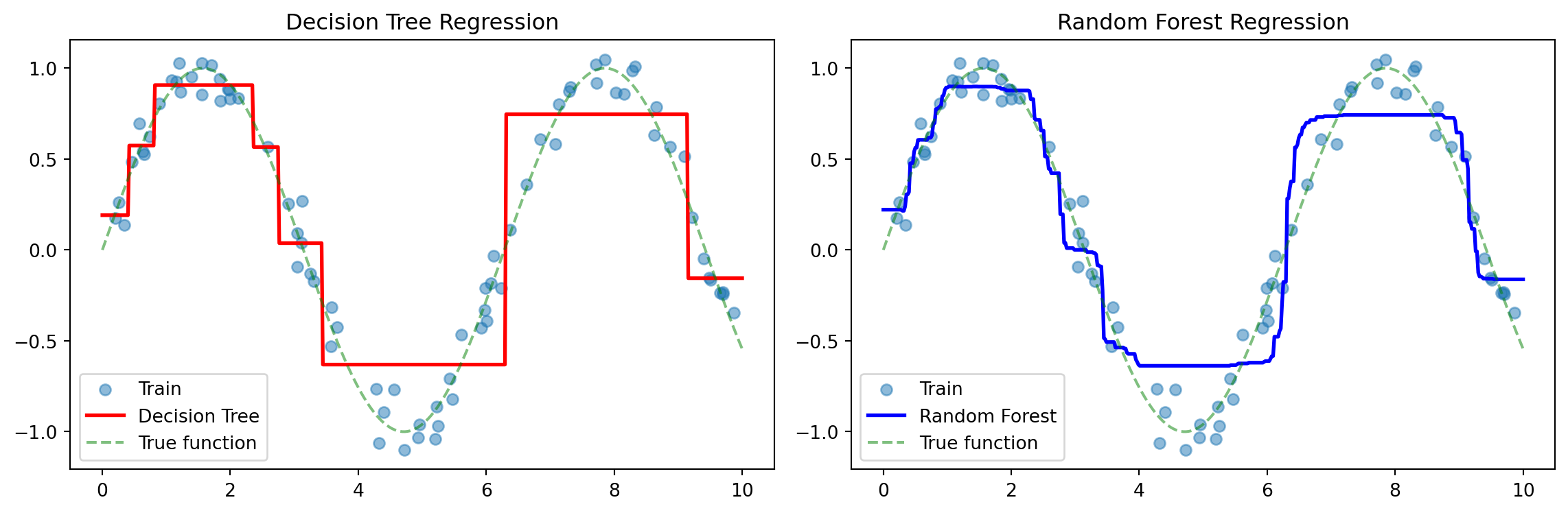
plt.figure(figsize=(12, 4))

plt.subplot(1, 2, 1)
plt.scatter(X_train, y_train, alpha=0.5, label='Train')
plt.plot(X_plot, y_dt, 'r-', linewidth=2, label='Decision Tree')
plt.plot(X_plot, np.sin(X_plot), 'g--', alpha=0.5, label='True function')
plt.legend()
plt.title('Decision Tree Regression')

plt.subplot(1, 2, 2)
plt.scatter(X_train, y_train, alpha=0.5, label='Train')
plt.plot(X_plot, y_rf, 'b-', linewidth=2, label='Random Forest')
plt.plot(X_plot, np.sin(X_plot), 'g--', alpha=0.5, label='True function')
plt.legend()
plt.title('Random Forest Regression')

plt.tight_layout()
plt.show()
Decision Tree R²: 0.883
Random Forest R²: 0.897
Decision Tree RMSE: 0.205
Random Forest RMSE: 0.193

Expected Output: - Decision Tree: Step-like predictions (piecewise constant) - Random Forest: Smoother predictions averaging many step functions

Example 8: Real-World Application - Housing Prices

Code
from sklearn.datasets import fetch_california_housing
from sklearn.preprocessing import StandardScaler

# Load data
housing = fetch_california_housing()
X, y = housing.data, housing.target

# Split
X_train, X_test, y_train, y_test = train_test_split(
    X, y, test_size=0.2, random_state=42
)

# Note: No need to scale features for tree-based methods!
# (But we would need to for linear regression)

# Train Random Forest
rf = RandomForestRegressor(
    n_estimators=100,
    max_depth=10,
    min_samples_split=10,
    random_state=42,
    n_jobs=-1  # Use all CPU cores
)

rf.fit(X_train, y_train)
y_pred = rf.predict(X_test)

print(f"R² Score: {r2_score(y_test, y_pred):.3f}")
print(f"RMSE: {np.sqrt(mean_squared_error(y_test, y_pred)):.3f}")

# Feature importance
importances = rf.feature_importances_
features = housing.feature_names

for name, imp in sorted(zip(features, importances), 
                        key=lambda x: x[1], 
                        reverse=True):
    print(f"{name}: {imp:.3f}")
R² Score: 0.773
RMSE: 0.545
MedInc: 0.600
AveOccup: 0.140
Latitude: 0.076
Longitude: 0.076
HouseAge: 0.047
AveRooms: 0.030
AveBedrms: 0.016
Population: 0.016

Interpretation: Feature importance shows which variables matter most for prediction. This is a huge advantage over linear regression where coefficient interpretation can be tricky.

When to Use Which Method?

Use Decision Trees when:

  • ✓ Interpretability is crucial
  • ✓ You have limited data
  • ✓ You need a quick baseline model
  • ✓ Features are mostly categorical

Use Random Forests when:

  • ✓ Predictive accuracy is the priority
  • ✓ You have enough data (100+ samples)
  • ✓ The relationship is complex/non-linear
  • ✓ You need feature importance rankings
  • ✓ You want robust predictions with less tuning

Use Linear Regression when:

  • ✓ The relationship is truly linear
  • ✓ You need to extrapolate beyond training data
  • ✓ You need smooth predictions
  • ✓ Coefficient interpretation is important

Key Takeaways

  1. Decision trees partition the feature space into rectangles and predict the average within each region
  2. Splitting is done greedily to minimize variance (RSS) in resulting groups
  3. Single trees are interpretable but prone to overfitting and instability
  4. Random forests build many diverse trees through bootstrapping and random feature selection
  5. Averaging predictions reduces variance while maintaining the trees’ ability to capture non-linearity
  6. No feature scaling needed for tree-based methods
  7. Feature importance is automatically computed and very useful
  8. Hyperparameter tuning is important but random forests are fairly robust to default settings

Summary

Decision tree and random forest regression are powerful tools in the data scientist’s toolkit. They handle non-linearity naturally, require minimal preprocessing, and provide excellent predictive performance. While single trees offer interpretability, random forests sacrifice some interpretability for superior accuracy and robustness. Understanding when and how to use these methods will significantly expand your regression modeling capabilities.

Back to top