Causal Inference II: Causal Graphs and Estimating Effects

In Causal Inference I we saw that the naive difference in means equals the true effect plus selection bias, and that randomization removes that bias. But we often cannot run an experiment:

• it would be unethical (randomly assign people to smoke),
• it is impossible (we can’t re-run a minimum-wage law),
• it is too expensive or slow, or
• the treatment already happened and we only have observational data.

This lecture is about doing causal inference without an experiment — which forces us to be explicit about our assumptions using causal graphs.

Drawing our assumptions: causal graphs

A causal graph is a directed acyclic graph (DAG): nodes are variables, and an arrow \(X \rightarrow Y\) means “\(X\) is a direct cause of \(Y\)” (Pearl et al. 2016).

The graph encodes assumptions we bring to the data (from domain knowledge). The data alone cannot draw it for us — but once drawn, the graph tells us exactly which variables to control for.

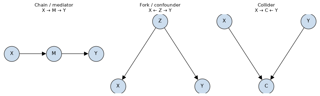
Remarkably, every DAG is built from just three elementary structures.

The three building blocks

• Chain \(X \to M \to Y\): \(M\) is a mediator (it transmits the effect).
• Fork \(X \leftarrow Z \to Y\): \(Z\) is a confounder (common cause).
• Collider \(X \to C \leftarrow Y\): \(C\) is a common effect.

The golden rule: adjust for forks, not colliders

The three structures behave oppositely when you condition (adjust/stratify) on the middle node:

Structure	Middle node	Adjust for it?	Why
Fork \(X \leftarrow Z \to Y\)	confounder	Yes	blocks the spurious backdoor path
Chain \(X \to M \to Y\)	mediator	No*	it’s part of the effect you want
Collider \(X \to C \leftarrow Y\)	collider	No!	conditioning creates spurious association

* Adjust for a mediator only if you specifically want the direct (not total) effect.

“Just throw every variable into the regression” is wrong — controlling for a collider or a mediator introduces bias. Choosing controls is a causal decision, not a statistical one (Cinelli et al. 2024).

Confounders: the backdoor

A backdoor path is a non-causal path from \(X\) to \(Y\) that starts with an arrow into \(X\) (e.g. \(X \leftarrow Z \to Y\)). Backdoor paths are the graph-language for confounding.

Backdoor criterion: a set of variables \(S\) suffices to identify the causal effect of \(X\) on \(Y\) if \(S\) blocks every backdoor path and contains no descendants of \(X\) (Pearl 2009).

When such an \(S\) exists and we adjust for it, we get the adjustment formula: \[ P(Y \mid do(X{=}x)) = \sum_{s} P(Y \mid X{=}x, S{=}s)\, P(S{=}s). \] This is the formal justification for “controlling for confounders.”

Colliders: adjusting can create bias

Conditioning on a collider (or its descendant) opens a spurious path. Classic example: suppose talent and looks are independent in the general population, but both help an actor get famous.

import numpy as np
rng = np.random.default_rng(701)
n = 10_000

talent = rng.normal(0, 1, n)
looks  = rng.normal(0, 1, n)          # independent of talent by construction
famous = (talent + looks + rng.normal(0, 0.5, n)) > 1.5   # collider: common effect

corr_all    = np.corrcoef(talent, looks)[0, 1]
corr_famous = np.corrcoef(talent[famous], looks[famous])[0, 1]
print(f"corr(talent, looks) overall        = {corr_all:+.2f}")
print(f"corr(talent, looks) among famous    = {corr_famous:+.2f}")

corr(talent, looks) overall        = +0.00
corr(talent, looks) among famous    = -0.55

Among the famous, talent and looks are negatively correlated — “why are talented celebrities so often unattractive?” — even though they are unrelated in general. We manufactured the correlation by conditioning on fame. This is collider / selection bias (a.k.a. Berkson’s paradox).

Mediators: don’t “control away” your effect

If a job-training program raises earnings by teaching skills:

\[ \text{Training} \rightarrow \text{Skills} \rightarrow \text{Earnings} \]

Controlling for skills would block the very pathway the program works through, making the program look useless. This is overcontrol bias.

Rule of thumb for a total effect: adjust for common causes, never for anything on the causal path or for common effects (Cinelli et al. 2024).

Estimating effects under “no unmeasured confounders”

Suppose we’ve drawn the DAG and found an adjustment set \(S\) that satisfies the backdoor criterion (the ignorability / unconfoundedness assumption). Several estimators then recover the effect:

1. Regression adjustment — include \(S\) as covariates; read off the coefficient on \(T\).
2. Stratification / standardization — estimate the effect within levels of \(S\), then average (weighting by the population, not the treated group).
3. Matching — pair each treated unit with similar control unit(s) on \(S\).
4. Propensity scores — match or weight on \(e(S) = P(T{=}1 \mid S)\), a one-number summary.

Regression vs. stratification, side by side

import numpy as np, pandas as pd, statsmodels.formula.api as smf

rng = np.random.default_rng(0)
n = 4000
# Confounder Z drives BOTH treatment and outcome
Z = rng.normal(0, 1, n)
T = (rng.uniform(size=n) < 1 / (1 + np.exp(-Z))).astype(int)   # sicker -> treated
Y = 3.0 * T + 2.0 * Z + rng.normal(0, 1, n)                    # TRUE effect = 3.0
df = pd.DataFrame({"Y": Y, "T": T, "Z": Z})

naive = smf.ols("Y ~ T", data=df).fit().params["T"]
adj   = smf.ols("Y ~ T + Z", data=df).fit().params["T"]
print(f"True effect        = 3.00")
print(f"Naive (ignore Z)   = {naive:.2f}   <- biased")
print(f"Adjusted (+ Z)     = {adj:.2f}   <- recovers truth")

True effect        = 3.00
Naive (ignore Z)   = 4.65   <- biased
Adjusted (+ Z)     = 3.00   <- recovers truth

Adjusting for the confounder \(Z\) recovers the true effect of \(3.0\); ignoring it does not. Same idea as stratifying the kidney-stone table — just done with a regression.

Propensity scores in one slide

When \(S\) is high-dimensional, matching directly is hard. Rosenbaum & Rubin showed it is enough to match/weight on the scalar propensity score \(e(S) = P(T{=}1\mid S)\).

from sklearn.linear_model import LogisticRegression

# Estimate propensity, then inverse-propensity weighting (IPW) for the ATE
ps = LogisticRegression().fit(df[["Z"]], df["T"]).predict_proba(df[["Z"]])[:, 1]
w = np.where(df["T"] == 1, 1 / ps, 1 / (1 - ps))
ate_ipw = (np.sum(w * df["T"] * df["Y"]) / np.sum(w * df["T"])
           - np.sum(w * (1 - df["T"]) * df["Y"]) / np.sum(w * (1 - df["T"])))
print(f"IPW estimate of ATE = {ate_ipw:.2f}   (true = 3.0)")

IPW estimate of ATE = 3.03   (true = 3.0)

Inverse-propensity weighting builds a “pseudo-population” in which treatment is unrelated to \(S\) — mimicking a randomized experiment from observational data.

When confounders are unobserved: natural experiments

Adjustment only works for confounders we can measure. When we can’t, we look for “nature’s randomization” — sources of variation in treatment that are as good as random (Angrist and Pischke 2014).

Three workhorse designs:

• Difference-in-Differences (DiD),
• Instrumental Variables (IV),
• Regression Discontinuity (RD).

Difference-in-Differences

Compare the change in a treated group to the change in a control group over time. This differences out any fixed differences between the groups.

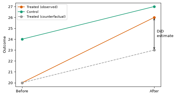
Card & Krueger’s famous study used DiD to show a New Jersey minimum-wage increase did not reduce fast-food employment relative to neighboring Pennsylvania (Card and Krueger 1994). Key assumption: parallel trends (absent treatment, both groups would have moved together).

Instrumental variables & regression discontinuity

Instrumental variable (IV)

An instrument \(Z\) affects the outcome only through the treatment: \[ Z \rightarrow T \rightarrow Y, \quad Z \not\rightarrow Y \text{ directly}. \]

• Vietnam draft lottery as an instrument for military service.
• Distance to college as an instrument for years of schooling.

\(Z\) acts like the coin flip we wish we had run.

Regression discontinuity (RD)

Treatment switches on at a cutoff of a running variable. Units just above vs. just below are comparable.

• Scholarship awarded at a test-score threshold.
• Class-size caps that trigger a new section.

Compare outcomes in a narrow window around the cutoff.

All three designs trade the “no unmeasured confounders” assumption for a different, often more credible, assumption. There is no free lunch — every causal estimate rests on assumptions that data cannot fully verify.

Assumptions you can’t skip

Every observational causal estimate relies on assumptions (Hernán and Robins 2020):

• Unconfoundedness / ignorability — all confounders in the adjustment set are measured.
• Positivity (overlap) — every unit has a nonzero chance of each treatment (\(0 < e(S) < 1\)).
• SUTVA — one unit’s treatment doesn’t affect another’s outcome (no interference), and there’s a single version of the treatment.
• Correct graph — the DAG reflects reality.

Since unconfoundedness is untestable, good practice includes a sensitivity analysis: how strong would an unmeasured confounder have to be to overturn the conclusion?

Tools and the modern workflow

• DoWhy — model (DAG) → identify → estimate → refute; a clean four-step API (Sharma and Kiciman 2020).
• EconML — ML-based heterogeneous treatment effects (CATE).
• dagitty — draw a DAG in the browser; it tells you the valid adjustment sets.
• Classical estimators live in statsmodels, scikit-learn, and linearmodels.

The workflow is always: draw the graph → identify an estimand → estimate → challenge it with robustness checks. The graph comes first.

Recap

• A DAG encodes causal assumptions; every DAG is chains, forks, and colliders.
• Adjust for confounders (forks); do not adjust for mediators or colliders — bad controls create bias.
• The backdoor criterion tells you a valid adjustment set; the adjustment formula, regression, stratification, matching, and propensity scores then estimate the effect.
• When confounders are unmeasured, use natural experiments — DiD, IV, RD.
• Every estimate rests on untestable assumptions (ignorability, positivity, SUTVA); state them and stress-test them.

Small-Group Activity

🎯 Activity: Be the causal analyst (≈30 min)

Format: groups of 3–4. Time: ~20 min of group work + ~10 min report-out.

You will get a scenario. For it, your group must produce four deliverables:

1. Define the treatment \(T\), the outcome \(Y\), and the target estimand (ATE? ATT? CATE?).
2. Draw a DAG with at least one plausible confounder, one mediator, and one collider. Label each.
3. Identify what you would adjust for, and — just as important — what you would not adjust for, and why (name the backdoor path / the collider you’re avoiding).
4. Choose a strategy: an experiment (how would you randomize?) or an observational design (regression/matching/propensity, or DiD/IV/RD). State the key assumption it relies on and one way it could fail.

Choose a scenario

Pick one (or your instructor will assign one):

A. Product / tech

Does adding a “free shipping” badge on product pages increase purchases? You have historical logs; badges were shown more often on popular items.

B. Health

Does a new fitness-tracking app reduce users’ resting heart rate? People who download it are already more health-conscious.

C. Education

Does an optional tutoring program raise final grades? Students self-select into tutoring, and struggling students are more likely to sign up.

D. Policy

Does a city’s new bike-lane network reduce traffic accidents? It was built in denser, wealthier neighborhoods first.

Watch for the trap in each: the variable that is tempting to “control for” but is actually a mediator or collider. Find it and justify your choice.

Report out

Each group takes ~2 minutes to share:

1. your DAG (sketch it on the board / share your screen),
2. the one variable you deliberately did not adjust for, and why,
3. your identification strategy and its weakest assumption.

Discussion prompts for the whole class:

• Where did groups disagree about the DAG? Whose assumption is more defensible?
• Which scenarios are best served by an experiment vs. an observational design?
• For your scenario, what data would most change your confidence in the estimate?

References

• Causal Inference: What If — Hernán & Robins (free PDF)
• Causal Inference: A Primer — Pearl, Glymour & Jewell
• “A Crash Course in Good and Bad Controls” — Cinelli, Forney & Pearl
• DoWhy documentation and dagitty.net

Bibliography

Angrist, Joshua D., and Jörn-Steffen Pischke. 2014. Mastering ’Metrics: The Path from Cause to Effect. Princeton University Press.

Card, David, and Alan B. Krueger. 1994. “Minimum Wages and Employment: A Case Study of the Fast-Food Industry in New Jersey and Pennsylvania.” American Economic Review 84 (4): 772–93.

Cinelli, Carlos, Andrew Forney, and Judea Pearl. 2024. “A Crash Course in Good and Bad Controls.” Sociological Methods & Research 53: 1071–104. https://doi.org/10.1177/00491241221099552.

Hernán, Miguel A., and James M. Robins. 2020. Causal Inference: What If. Chapman & Hall/CRC. https://www.hsph.harvard.edu/miguel-hernan/causal-inference-book/.

Pearl, Judea. 2009. Causality: Models, Reasoning, and Inference. 2nd ed. Cambridge University Press.

Pearl, Judea, Madelyn Glymour, and Nicholas P. Jewell. 2016. Causal Inference in Statistics: A Primer. Wiley.

Sharma, Amit, and Emre Kiciman. 2020. DoWhy: An End-to-End Library for Causal Inference. https://arxiv.org/abs/2011.04216.